Research symposium
A Tale of Two ValleysThe Hidden Geometry of Excitons
Can we have topological excitons in biased bilayer graphene?
Exciton Berry curvature from a finite-momentum Bethe–Salpeter calculation
Sviatoslav Gladyshev
Supervisor: Dr. Marwa Mannai
Center for Quantum and Topological Systems, NYU Abu Dhabi · Ateno
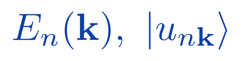
[0:25] Good afternoon. In this talk, the two valleys are K and K-prime in bilayer graphene, and the hidden geometry is the Berry curvature of the excitons that form there. The question I have been working on with Dr. Marwa Mannai is in blue: can we have topological excitons in biased bilayer graphene?
For questions: The title borrows from Dickens, A Tale of Two Cities.
By topological excitons I mean Berry curvature or topology of the exciton states themselves, as functions of the exciton's centre-of-mass momentum Q, not the well-known topology of the electron bands.
Plan: devices that already move excitons and polaritons; the electrons of biased bilayer graphene; exciton theory; my own calculation (slides 14-19); possible applications. Throughout I keep apart established physics, published results by others, my own model results, and open questions.
Bound.
An electron and a hole, held by Coulomb attraction. Approximately a boson at low density.
Neutral.
No net charge current, yet energy and information still move.
Geometric.
Their motion may depend on the geometry of the exciton band.
Hypothesis: if the composite has its own band geometry, an electric field could steer how it moves.
2
An exciton is an electron and a hole bound together, so it carries energy but no net charge. That makes it hard to steer with an ordinary voltage. Our hypothesis is that the geometry of the exciton band gives another handle on its motion, and that hypothesis is untested here.
Motivation · devices that exist today
Excitons and polaritons already carry information. Optoexcitonic switch
Gated flow
WSe₂ monolayer · room temperature
Takeaway: excitons can be guided and switched like a signal.
Not: topological, and not graphene.
Jiang et al., ACS Nano 19, 32123 (2025)
Polariton transistor
2 × 2 µm²
Polymer in silicon-photonics cavities · room temperature
Takeaway: polaritons switch and amplify light on a chip, in picoseconds.
Not: bare excitons; not topological.
Tassan et al., Light Sci. Appl. 15, 65 (2026)
Polariton spin logic
60 µm
Perovskite (FAPbBr₃) microcavity · room temperature
Takeaway: polariton spin travels 60 µm and drives a logic gate.
Not: exciton Berry curvature: photonic spin–orbit coupling.
Shi et al., Nat. Mater. 24, 56 (2025)
Valley routing
gap ≈ 9 meV
Patterned perovskite valley-Hall lattice · room temperature
Takeaway: K and K′ states can be routed in opposite directions.
Not: excitonic topology: the lattice is engineered.
Jin et al., Nat. Commun. 15, 10563 (2024)
All four are working experiments. None is bilayer graphene, and none uses the Berry curvature of the excitons themselves.
Published experiments
3
[0:55] Excitons, and polaritons, which are excitons mixed with light, already carry information in the lab. Here are four room-temperature experiments.
(Left to right.) Excitons in a WSe₂ monolayer, guided along a channel and switched by a gate. A polariton transistor on a chip that switches and amplifies light in picoseconds. Polariton spin carried sixty microns and used in a logic gate. And valley routing, where K and K-prime states travel in opposite directions.
(Point to the tags.) Three of the four are polaritons, none is bilayer graphene, and none uses the Berry curvature of the excitons themselves. That is where my work fits.
For questions: Jiang et al., ACS Nano 2025 (Michigan): bare excitons in a WSe₂ monolayer pushed along a one-dimensional guide by a light-engineered force and switched by a gate.
Tassan et al., Light Sci. Appl. 2026 (IBM Research Zurich and collaborators): a polymer in silicon-photonics cavities, 2 × 2 µm², picosecond switching, amplification up to 60×.
Shi et al., Nat. Mater. 2025: perovskite microcavity; circular polarization (the polariton spin) travels 60 µm; a NOT gate and a spin-polarized beam splitter.
Jin et al., Nat. Commun. 2024: patterned perovskite valley-Hall lattice; topological kink states, gap about 9 meV; K and K′ states propagate in opposite directions. The topology is engineered into the photonic lattice, not intrinsic to the excitons.
Motivation · spin currents in polariton waveguides
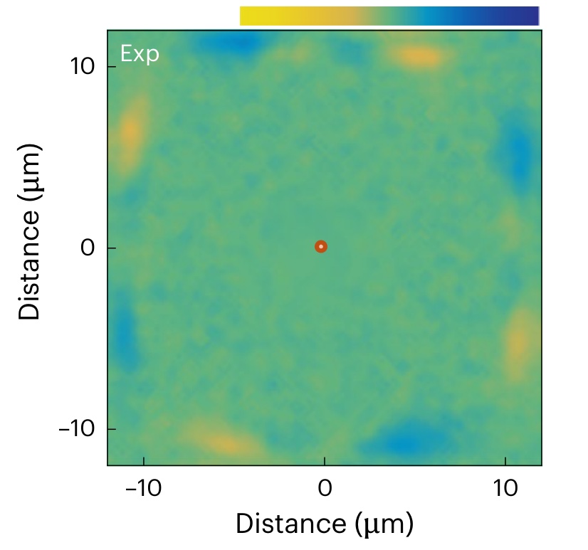
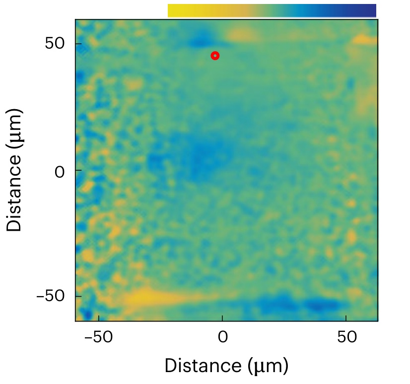
Spin information travels 92 µm at room temperature. Eight spin domains around the pump (red dot), 20 × 20 µm² cavitySpin across the cavity , 100 × 100 µm², pump near the top edgeColour: degree of circular polarization, yellow σ⁺ to blue σ⁻. Measured, hBN/WS₂/SiN/SiO₂.
92 µm
spin-polarized polariton transport at room temperature, with ordinary non-resonant pumping
1
Bright excitons in WS₂ mix with guided light into long-lived, fast polaritons.
2
Dark excitons , filled by ordinary pumping, act as a built-in source for both TE and TM modes.
3
Optical spin Hall effect: TE–TM splitting of the light modes turns linear into circular polarization.
Why it matters: long-range spin transport at room temperature is a step towards spin-polaritonic logic circuits.
Different physics from ours: the spin texture comes from photonic TE–TM splitting in a WS₂ waveguide, not from exciton Berry curvature, and not from bilayer graphene. It motivates applications; it does not test our mechanism.
Experiment · WS₂
Figure: Research Briefing, Nat. Mater. (2026) , © 2026 Shang, Q. et al. · Paper: Q. Shang et al., Nat. Mater. (2026)
4
[1:15] This is the paper Dr. Mannai recommended, by Shang and colleagues in Nature Materials. The headline: spin-polarized polaritons travel ninety-two microns at room temperature, with an ordinary off-resonant laser.
(Point to the steps.) Three ingredients. First, bright excitons in a WS₂ monolayer mix with light in a waveguide and form long-lived, fast polaritons. Second, WS₂ also has dark excitons. Ordinary pumping fills them, and they act as a built-in source for both TE and TM guided modes. Third, TE and TM modes propagate differently, which turns linear polarization into circular: the optical spin Hall effect. (Point to the maps.) That gives these eight spin domains, and spin reaching across a hundred-micron cavity.
Long-range spin transport at room temperature is a step towards spin-polaritonic logic. (Orange box.) But the mechanism is the spin–orbit coupling of light in WS₂. It is not exciton Berry curvature, and it does not test my calculation. It is motivation.
For questions: Shang et al., Nat. Mater. (published 2 November 2026), with a research briefing by Zúñiga-Pérez and Malpuech. Spin-polarized polariton currents propagate 92 ± 1 µm at room temperature, with non-resonant pumping and a degree of circular polarization above 75 %. The briefing says this is one to two orders of magnitude further than electron spins travel, while the polaritons keep their nonlinearity.
Bright excitons have in-plane dipoles and couple to the guided modes of a SiN waveguide; the photons are below the light cone, so the polaritons live longer and move faster than in a vertical cavity.
Dark excitons have out-of-plane dipoles at lower energy. Under off-resonant pumping they act as a linearly polarized source that feeds a coherent superposition of quasi-TE and quasi-TM modes; normally that needs resonant excitation or a condensate.
Applications proposed by the authors: concatenated spin logic gates and integrated spin-polaritonic circuits; still missing are spin amplifiers and memories.
Figure from the Nature Materials research briefing, © the authors.
Motivation · why biased bilayer graphene?
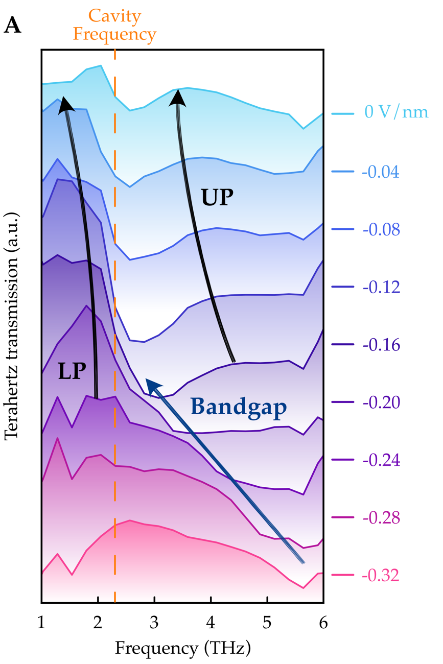
Bilayer graphene already works inside a cavity. Experiment
Bilayer graphene
Dual-gated AB bilayer in a terahertz cavity
The gate field D tunes the gap through the cavity frequency. Ultrastrong coupling, g/ωc ≈ 40 %.
A cavity-induced, exciton-like state is pulled out of the electron–hole continuum (LP).
Not: our exciton. Photon-mediated binding at meV gaps and 5 K, not Coulomb excitons.
Helmrich et al., Nature 654, 361 (2026)
Theory
Biased bilayer graphene
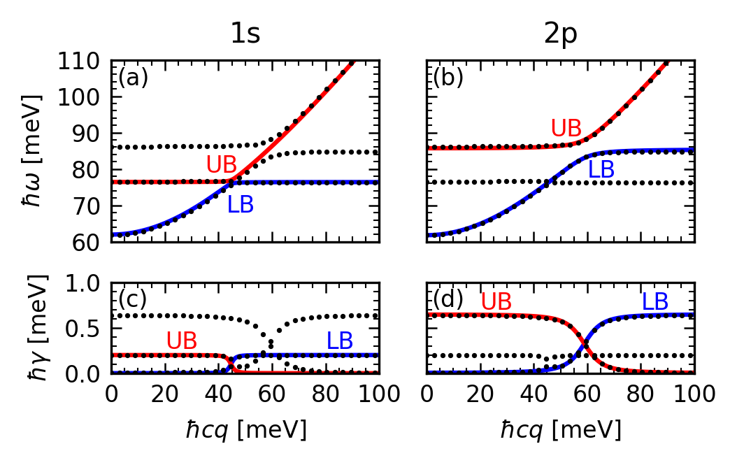
Exciton-polaritons tuned by the bias
The bias tunes the polariton branches (UB, LB) and the Rabi splitting. Shown at 100 meV, the bias used in our model.
Not: measured yet, and no exciton geometry.
Duarte et al., Phys. Rev. B 111, 075411 (2025)
Experiment: the platform exists. Theory: the bias tunes its polaritons. Missing: the geometry of the exciton states themselves.
Figures: Helmrich et al., arXiv:2408.00189 version, n = 0, 5 K (CC BY 4.0) · Duarte et al., arXiv:2502.06640, Fig. 4 (CC BY 4.0)
5
[0:45] Why bilayer graphene? Because a gate tunes its band gap, and it already works in a cavity.
(Left.) This year, a group at ETH Zürich put gated bilayer graphene in a terahertz cavity and reached ultrastrong coupling. The cavity even creates an exciton-like state, but that binding comes from photons, at five kelvin, so it is not our exciton. (Right.) Duarte and colleagues predict exciton-polaritons whose branches are tuned by the bias, at the same hundred milli-electron-volts I use.
What is missing is the geometry of the exciton states themselves.
For questions: Helmrich et al., Nature 654, 361 (2026), ETH Zürich: dual-gated AB bilayer under a terahertz bow-tie resonator. The displacement field tunes the gap through the cavity frequency; coupling about 40 % of the photon frequency. A cavity-induced, exciton-like state (LP) is pulled out of the electron–hole continuum. The binding is photon-mediated, at gaps of a few meV and 5 K; ordinary Coulomb excitons were not resolved.
Duarte et al., Phys. Rev. B 111, 075411 (2025): theory of exciton-polaritons in biased bilayer graphene in an optical microcavity; the bias changes the exciton energy, the Hopfield mixing and the Rabi splitting. Excitons enter through a fitted Elliott model, with no geometry. Not yet measured.
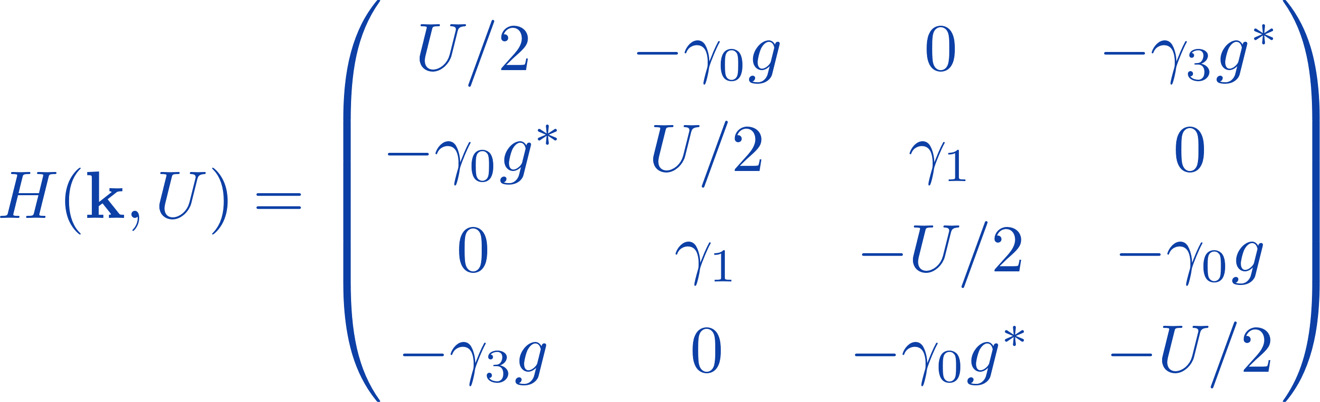
Biased bilayer graphene · 1 · the Hamiltonian
Four orbitals and one gate-controlled bias. A₁ B₁ A₂ B₂ γ₀ γ₀ γ₁ γ₃ +U/2 −U/2 layer 1 layer 2 E field A₁, B₁ · A₂, B₂
carbon pz orbitals of the top and bottom layers
γ₀ = 3.0 eV
in-plane nearest-neighbour hopping
γ₁ = 0.40 eV
vertical B₁–A₂ (dimer) coupling
γ₃ = 0.30 eV
skew A₁–B₂ hopping: trigonal warping
±U/2
layer potentials from the gate: the only place the bias U enters
Established model
Basis (A₁, B₁, A₂, B₂) · lattice form used for the whole Brillouin zone · Appendix A: continuum form and derivations
6
[1:10] To get there, we need the electrons first. (Point to the diagram.) AB bilayer graphene has four carbon sites per unit cell: A1 and B1 in the top layer, A2 and B2 in the bottom. Each site contributes one p-z orbital, so the tight-binding Hamiltonian is four by four.
Gamma-zero, three electron-volts, is the in-plane hopping. Gamma-one, 0.4 electron-volts, couples B1 and A2, which sit directly on top of each other. Gamma-three is a weaker skew hopping that warps the bands. The gate enters in one place only: a potential of plus U over two on the top layer and minus U over two on the bottom.
I use the lattice form over the whole Brillouin zone, because the exciton calculation involves both valleys. Near K it reduces to the familiar continuum model.
For questions: g(k) is the sum over the three nearest-neighbour vectors of exp(ik·δ). Near K, g ≈ −(√3a/2)(pₓ − ip_y), and the matrix reduces exactly to the continuum Hamiltonian; the code checks this numerically to 10⁻¹¹ eV.
The whole-zone form is needed because the screening and exchange sums run over the entire zone, including both valleys.
This is the established tight-binding model of McCann and Koshino; the parameters are standard values, not fitted to a device. Continuum derivations are in Appendix A.
Biased bilayer graphene · 3 · electronic topology
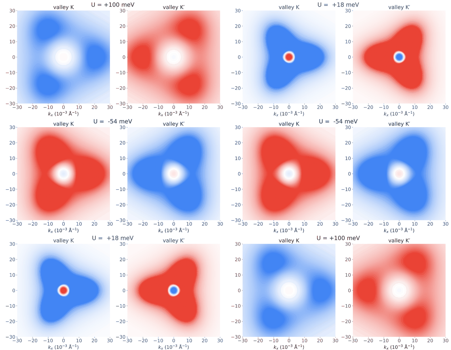
Electronic Berry curvature flips with the bias.
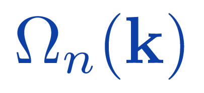
Electronic Berry curvature Ω(k) acts like a magnetic field in momentum space for one Bloch band. Integrated over one valley, it gives the valley Chern number.
conduction
K
K′
U > 0
−1
+1
U < 0
+1
−1
Opposite in K and K′, so the total Chern number is zero; reversing U reverses both.
This is electronic Berry curvature, in k. Exciton Berry curvature, in Q, is a separate calculation.
Author’s two-band model · U from +100 to −100 meV · blue: negative, red: positive · Appendix A: Chern derivation
8
Established physics · derived here
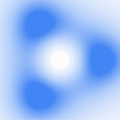
[1:30] Now the electronic topology. This is established physics, which I re-derived as my starting point. Electronic Berry curvature describes how the phase of a Bloch state changes as k goes around a small loop; it acts like a magnetic field in momentum space.
(Point to the animation.) Here it is concentrated near the band edge, it has three lobes because of trigonal warping, it is opposite in K and K-prime, and it flips sign when the bias reverses.
Integrating it over one valley gives the valley Chern number: minus or plus one, depending on the sign of U. The two valleys cancel, so the total Chern number is zero, but the valley difference reverses with the gate. That is the origin of valley Hall physics in this material. [cut if late] It also explains topological kink states at domain walls.
(Orange line.) All of this is about single electrons, in k. The exciton Berry curvature, as a function of the exciton momentum Q, has to be calculated separately.
For questions: Conduction band, two-band model: C(K) = −sgn U and C(K′) = +sgn U. Appendix A derives this and shows that trigonal warping does not change it. The valley difference is ±2 and reverses with the gate.
The animation is from my two-band model as U sweeps from +100 to −100 meV; blue is negative, red positive electronic Berry curvature.
Opposite signs in K and K′ follow from time-reversal symmetry; the sign change with U follows from layer inversion.
Schematic
The story, in one picture.
Schematic · illustrative · not a computed result · not to scale
9
Schematic
[0:45] This animation is a cartoon, not a calculation. Light excites an electron into the conduction band and leaves a hole behind. Their Coulomb attraction binds them into an exciton, which moves as one neutral object.
(As the exciton bends.) The sideways bend at the end is the question of this talk: does the exciton band have a Berry curvature that could deflect it?
For questions: The picture draws the electron in the top layer and the hole in the bottom layer for clarity. In the real calculation each exciton state is a superposition of many electron–hole configurations, including both layers and both valleys.
The animation is kept unchanged from the earlier version of the talk.
Excitons · what kind of particle?
A composite boson with its own momentum Q.
Bare exciton
Electron plus hole, bound by Coulomb attraction.
Approximately bosonic at low density, when pairs do not overlap. This talk is about these.
Exciton-polariton
Exciton strongly coupled to a confined photon.
Part light, part matter. It needs a cavity or similar structure, so its physics differs from a bare exciton.
Centre-of-mass momentum. Every pair in one exciton state shares the same total momentum.
Being bosonic does not imply condensation, topological order or fault-tolerant transport.
Established physics
10
[0:30] Two kinds of particle to keep apart. A bare exciton is the bound electron–hole pair; an exciton-polariton also mixes in a cavity photon, so its mass and lifetime are different. Today is about bare excitons.
The key variable is Q, the momentum of the whole pair. Exciton Berry curvature is defined in Q, not in the electron momentum k.
For questions: At low density, when pairs do not overlap, excitons behave approximately as bosons; at high density the fermionic constituents matter again.
Convention: electron at k + Q/2, valence state at k − Q/2, so the pair carries total momentum Q and k labels the relative motion. Each exciton state gives a band E_S(Q).
Bosonic statistics alone gives none of condensation, topological order or protected transport.
Excitons · the finite-Q Bethe–Salpeter equation
Solving for excitons at finite momentum Q. A superposition of electron–hole pairs, all with total momentum Q.
1 Independent electron–hole excitation energies
2 Screened Coulomb attraction Kd : binds the pair
3 Electron–hole exchange Kx : repulsive, couples K and K′
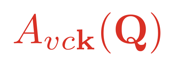
Output: exciton energies ES (Q) and wavefunctions AS (Q) . Exciton Berry curvature needs these weights and the Bloch states they multiply.
Why finite Q? Exciton Berry curvature describes how the exciton states change with Q, so the BSE is solved on a grid of Q around Q = 0.
Established method
Appendix B: exciton mathematics · Appendix C: kernels and screening used here
11
[1:20] To include electron–hole interactions, I solve the Bethe–Salpeter equation using the electronic states from the tight-binding Hamiltonian.
(Top line.) An exciton at momentum Q is a superposition of electron–hole pairs, with the electron at k plus Q over two and the hole at k minus Q over two. With two conduction and two valence bands there are four transitions at each k, and both valleys are in the same matrix.
(Second line.) The equation has three parts. First, the independent electron–hole excitation energies on the diagonal. Second, the screened Coulomb attraction, which binds the pair. Third, electron–hole exchange, which is repulsive and can move the pair between valleys, so it couples K and K-prime excitons.
(Right.) Why finite Q? Exciton Berry curvature describes how the exciton states change with Q, so I need solutions on a grid of Q around zero, not only at Q equals zero. (Box.) And the weights A alone are not enough: I also need the Bloch states they multiply.
For questions: First line: c† creates an electron in conduction band c at k + Q/2; c removes an electron from valence band v at k − Q/2, which leaves the hole. The coefficients A are the exciton wavefunction in the space of pairs.
Second line: Bethe–Salpeter equation in the Tamm–Dancoff approximation. Diagonal: E_c(k+Q/2) − E_v(k−Q/2). K^d: direct term, the screened attraction. K^x: exchange, the pair annihilating and re-creating; the factor 2 is for spin singlets.
Gauge: each A is defined relative to an arbitrary phase of each Bloch state, so the Berry curvature cannot be obtained from A alone; it needs A together with the Bloch states (slide 17).
The structure is the standard one (ABINIT, Sauer–Pedersen); the kernels I use are in Appendix C.
Excitons · published optics
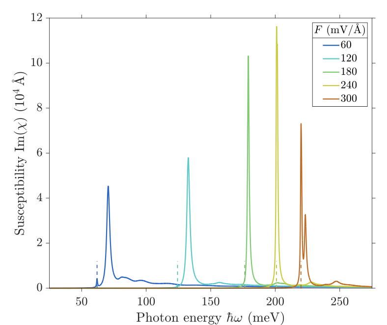
Bright, dark, and a field-driven crossing.
240 mV/Å
Dark and bright excitons swap order, in suspended and hBN-encapsulated samples alike. The crossing changes which state couples to light; on its own it is not a topological transition.
This work · model, U = 100 meV
Our lowest doublet is optically weak: ≈ 0.14 of the dipole strength of the brightest of the six lowest states (456-point check grid). No field sweep, so no crossing is claimed.
Dark states matter in devices too: out-of-plane dark excitons drive the WS₂ spin currents . Different material, different mechanism.
Figure: Sauer & Pedersen, Phys. Rev. B 105, 115416 (2022)
12
Published
[1:10] One more piece of published physics. Bright excitons couple to light; dark excitons do not. In bilayer graphene, the lowest exciton is mostly dark because of an angular-momentum selection rule. Sauer and Pedersen showed that near 240 millivolts per ångström a bright state moves below it. This crossing changes which state couples to light; on its own, it is not a topological transition.
(Box.) My model is consistent with the dark character: at my bias, the lowest pair has only about fourteen percent of the dipole strength of the brightest low-lying state. I did not sweep the field, so I make no claim about a crossing.
And a link back to WS₂: there, too, dark excitons turned out to matter, for a different microscopic reason.
For questions: Sauer and Pedersen, PRB 105, 115416 (2022): DFT-based Bethe–Salpeter calculation for biased bilayer graphene. Their figure shows absorption from 60 to 300 mV/Å. The crossing position is nearly the same for suspended and hBN-encapsulated samples. This is their result, not mine.
Selection rule: in the rotationally symmetric picture the band pseudospin contributes angular momentum ∓2 in K and K′, so a 1s exciton has total angular momentum ±2 and is dark, while normal-incidence light needs ±1; trigonal warping relaxes this weakly (Appendix B).
My number: ≈ 0.14 of the dipole strength of the brightest of the six lowest states, on a coarse 456-point check grid. Their field in mV/Å and my U are not directly interchangeable because of screening.
In WS₂ the dark state has an out-of-plane dipole that couples to TM-like waveguide modes; in bilayer graphene darkness comes from the angular-momentum selection rule.
Main results
Electronic valley Chern numbers are established.
Can we have topological excitons in biased bilayer graphene?
I calculated the Berry curvature of the exciton states themselves, as a function of the exciton momentum Q.
[0:15] So the electronic valley Chern numbers are established. The question is whether the excitons have Berry curvature of their own. The next six slides are my calculation.
For questions: Six slides: the calculation, the exciton energies, the exciton Berry curvature, why it is non-Abelian, the numerical checks, and the interpretation. Then one slide on possible applications.
Results · 1 · the numerical calculation
From the Hamiltonian to exciton Berry curvature. Numerical calculations implemented in Python
1
Tight-binding Hamiltonian
Four-orbital H(k, U) over the whole Brillouin zone
2
Diagonalize
Electronic energies and Bloch eigenstates
3
Finite-Q BSE Hamiltonian
Screened direct attraction + exchange
4
Solve
Exciton energies ES (Q) and wavefunctions
5
Lowest doublet
Two nearly degenerate excitons, isolated from the rest
6
Exciton Berry curvature
Non-Abelian, from gauge-covariant Wilson loops
≈ 8,000
coupled electron–hole configurations in the largest calculation, with both valleys in one Bethe–Salpeter matrix.
Model parameters (assumed, not a specific device)
γ₀ = 3.0 eV · γ₁ = 0.40 eV · γ₃ = 0.30 eV · a = 2.46 Å
This work · model calculation
Electron at k + Q/2, valence state at k − Q/2 · Appendix C: kernels, screening and conventions
14
[1:00] I implemented the numerical calculations in Python. (Point along the row.) First, I construct the four-orbital tight-binding Hamiltonian and diagonalize it to get the electronic energies and Bloch eigenstates. I then construct the finite-Q Bethe–Salpeter Hamiltonian, with screened direct attraction and exchange, and solve it for the exciton energies and wavefunctions. The largest calculation couples nearly eight thousand electron–hole configurations.
From the solutions I identify the lowest, nearly degenerate exciton doublet, and calculate its non-Abelian Berry curvature using gauge-covariant Wilson loops. (Right.) The parameters are standard model values, not a specific device.
For questions: Code: Python with NumPy and SciPy, written for this project (BLG_multiband_Berry).
Largest calculation: 1980 k points × 4 transitions = 7920 coupled electron–hole configurations, solved with an iterative block Davidson method and checked against dense diagonalization on a smaller grid.
The k grid covers the full zone and is much denser around K and K′, because the low-energy valleys are narrow; a coarse uniform grid gives wrong exciton energies.
Screening: static RPA polarization from the same electronic states, resolved by layer, so intra- and interlayer interactions are screened differently. Exchange for spin singlets with 19 reciprocal-lattice vectors (37 checked).
Parameters: γ₀ = 3.0, γ₁ = 0.40, γ₃ = 0.30 eV; a = 2.46 Å; U = +100 meV; κ = 4.5 (uniform dielectric environment); layer spacing 3.35 Å; Gaussian orbital radius 0.6 Å as a short-distance form factor. Neutral, T = 0; gates and anisotropic hBN are not modelled.
Results · 2 · exciton energies at Q = 0
The lowest excitons form a bound, nearly degenerate pair. free electron + hole 92.8 meV next exciton states lowest excitation · ≈ 70 meV two nearly degenerate states: K-like and K′-like ≈ 23 meV binding energy 9.3 meV to higher excitons When the exciton moves
its energy rises like a particle with mass, and the pair splits slightly.
70 75 80 -8 -4 0 +4 +8 momentum Qx (10⁻³ Å⁻¹) lowest pair next states 864 k points, so 70.8 meV at Q = 0
This work · model calculation
Model results, not measurements · ladder: 1980 BSE k points, screening on 5712 k
15
[1:00] The first result is the exciton energies. (Left.) The lowest excitation is at about seventy milli-electron-volts, and the binding energy is about twenty-three: the energy needed to separate the electron and hole. The lowest level is really two nearly degenerate states, one K-like and one K-prime-like, split by only about a nano-electron-volt.
The next exciton states are nine milli-electron-volts higher, so this pair is well separated from the rest. That separation is what lets me treat the pair as one well-defined subspace. (Right.) When the exciton moves, its energy rises like a particle with mass, and the two states split slightly.
For questions: Most refined run: 1980 k points in the BSE, screening on 5712 k points. Lowest exciton 70.016 meV; lowest free electron–hole pair on the same grid 92.790 meV; binding 22.77 meV relative to that discrete threshold, the consistent reference within this calculation.
Splitting of the doublet at Q = 0: 1.3 × 10⁻⁹ eV. The K-like and K′-like excitons are related by time reversal and mixed by exchange.
Separation to the next exciton: 9.32 meV at Q = 0, 9.25 meV including the corners of the standard Wilson loop, and at least 9.0 meV over the whole local map.
The right panel uses the 864-point grid, so it starts at 70.8 meV. Model results with assumed parameters; not measurements and not GW-corrected.
Results · 3 · exciton Berry curvature
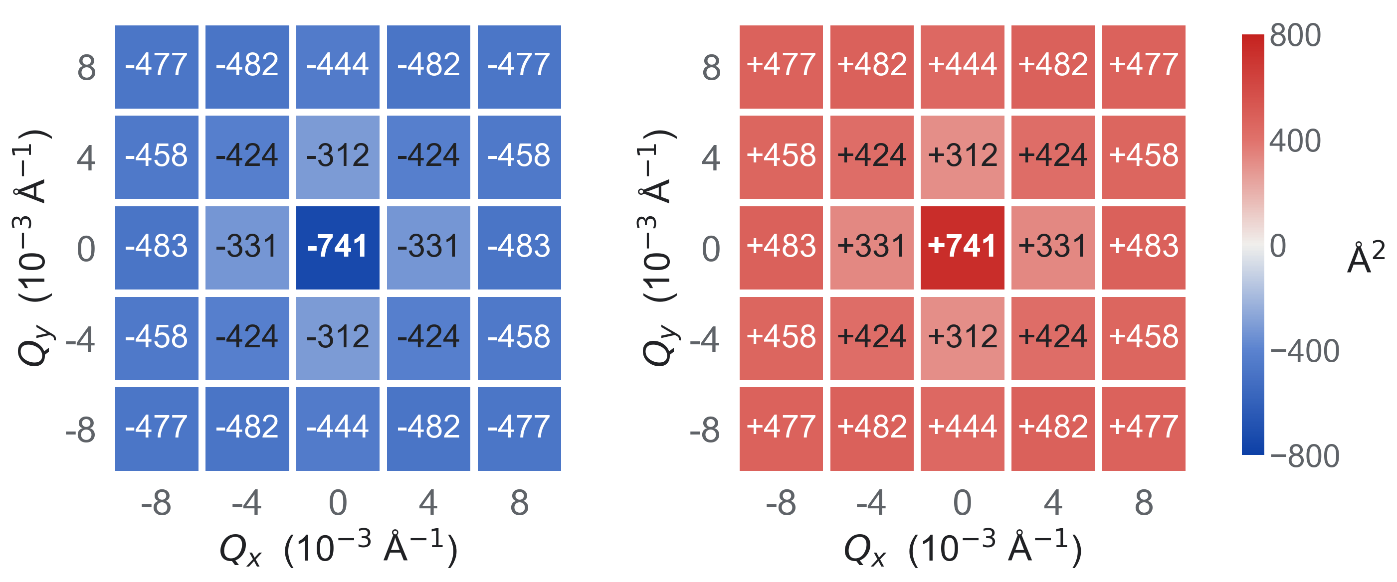
Opposite Exciton Berry Curvature in the Two Valleys Exciton Berry curvature near Q = 0
≈ ±730 Ų
Blue (−) and red (+) : opposite signsfor the K-like and K′-like states, each > 99.9 % in one valley.
Stronger colour = larger magnitude. Largest at Q = 0 (outlined).
The two lowest excitons are nearly degenerate, so their Berry curvature is calculated together. λ± are eigenvalues of their 2 × 2 Berry-curvature matrix, not Berry curvatures of two separate bands.
Calculated near Q = 0, not across the full exciton Brillouin zone.
Non-Abelian Berry-curvature eigenvalue λ− — K-like state
−8 Qx (10⁻³ Å⁻¹) +8
Non-Abelian Berry-curvature eigenvalue λ+ — K′-like state
−8 Qx (10⁻³ Å⁻¹) +8
−800 Ų exciton Berry curvature +800 Ų
Each tile is one calculated Q point (a small Wilson loop, 864 k points); colour set by its value. No interpolation.
This work · model calculation
Local map: lattice_local_map.npz · Bias reversal check · single states vs doublet
16
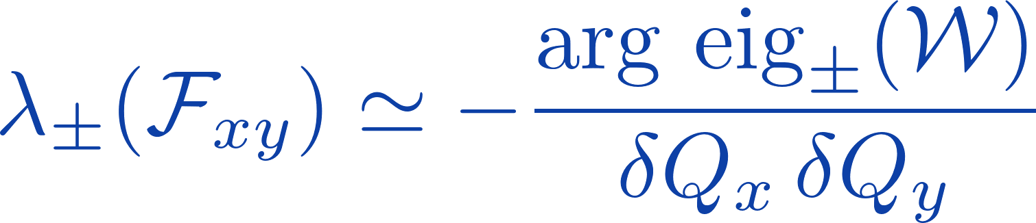
[1:30] This is the central result. (Point to the two maps.) Each tile is one Q point I calculated, and its colour is set by the calculated value. Blue means negative Berry curvature, red means positive, and stronger colour means a larger magnitude. The exciton Berry curvature is largest at Q equals zero, about seven hundred and thirty square ångström, and it has opposite signs in the two valleys.
The two lowest excitons are nearly degenerate, so their Berry curvature is calculated together. The result is a two-by-two Berry-curvature matrix, and its two eigenvalues, lambda-minus and lambda-plus, are the two maps. Each eigenvalue belongs to a state that is more than ninety-nine point nine percent in one valley: the left map is the K-like state, the right map the K-prime-like state. So the K-like and K-prime-like excitons have opposite Berry curvature, as time-reversal symmetry requires.
Two cautions. These are eigenvalues for a two-state subspace, not Berry curvatures of two separate bands. And the calculation covers a small region near Q equals zero, not the full exciton Brillouin zone.
For questions: Most refined value at Q = 0: λ∓ = ∓733.85 Ų (1980 k points, smallest Wilson loop, side 3.75 × 10⁻⁴ Å⁻¹). I quote ≈ 730 Ų because the numerical uncertainty is much larger than the last digits.
The map: 5 × 5 points with |Qₓ|, |Q_y| ≤ 0.008 Å⁻¹, under 0.7 % of Γ–K even at the corners, on the 864-point grid, hence 741 Ų at the centre. Off-centre values 312–483 Ų. Tile colours are the calculated values on a fixed ±800 Ų scale; no interpolation between points.
Valley polarization of the two eigenvectors: +0.999912 (λ₋, K) and −0.999912 (λ₊, K′), measured at Q = 0.
Scale: √734 Ų ≈ 27 Å, a length of the order of the exciton size here.
Bias reversal U → −U (456-point grid only): the same pair of values, with the valley assignment swapped. Links on the slide: bias reversal check and single states vs doublet (Appendix C).
Results · 4 · non-Abelian Berry curvature
Because the two lowest excitons are nearly degenerate, we calculate the Berry curvature of their combined subspace. Exciton overlap between neighbouring Q: BSE weights × electron and hole Bloch-state overlaps, so arbitrary phases cancel.
Q₁ Q ≈ 0 Q₂ same smooth plane: span{X₁, X₂} One energy state: jumps between nearby Q.
Two-state subspace: smooth everywhere.
The Wilson loop W gives the 2 × 2 Berry-curvature matrix F . A U(2) basis change inside the doublet only rotates W and F : λ± are basis-independent.
Two-state subspace
Berry-curvature eigenvalues λ± ≈ ±730 Ų
Single energy branches
Berry curvature compatible with zero
This work · model calculation
Appendix C: overlap diagnostics · Schematic on the left; values from lattice_local_map.npz
17
[1:00] Why calculate the Berry curvature of the pair? Because the two states are nearly degenerate, a single energy eigenstate is not a smooth function of Q. (Point to the discs.) A tiny step in Q can rotate the lowest state almost entirely into the other one, so its own Berry phase is ill-defined. The two-state subspace, the green disc, changes smoothly.
(Top.) So I compute overlaps between exciton states at neighbouring Q, including the electron and hole Bloch states, so arbitrary phases cancel. Multiplying them around a small square gives a Wilson loop, and its eigenphases give the Berry-curvature eigenvalues. (Box.) The subspace gives about plus and minus seven hundred and thirty square ångström; the single energy branches give Berry curvature compatible with zero.
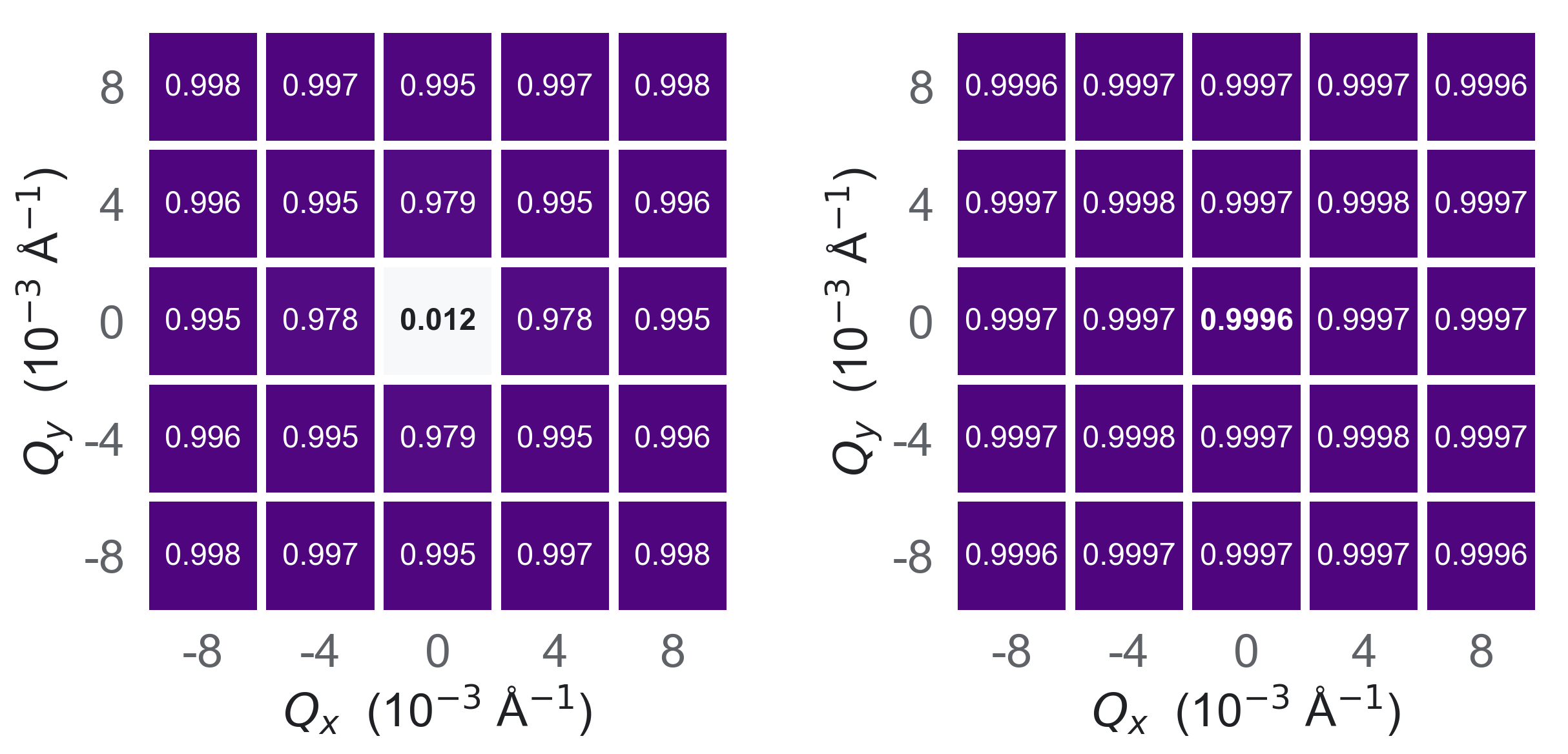
For questions: Overlap diagnostics: around the smallest loop at Q = 0, the overlap of the lowest energy state with itself drops to 0.012, so its Abelian Berry phase is meaningless there. For the two-state subspace, the smallest singular value of the overlap matrix M is at least 0.9996 everywhere on the map.
M_ST(Q,Q′) = BSE weights of the two states × electron Bloch overlap (k+Q/2, k+Q′/2) × valence Bloch overlap (k−Q′/2, k−Q/2), summed over band pairs. Differentiating A directly would give a gauge-dependent answer.
From each M take the closest unitary via the SVD and multiply around a small square: the Wilson loop W. With A = i⟨X|∇_Q X⟩, the eigenphases of W divided by the loop area give the eigenvalues of the Berry-curvature matrix F_xy. A U(2) rotation inside the doublet conjugates W and F, so the eigenvalues are basis-independent; tested with random U(2) rotations.
Single exchange-mixed branches, away from the central degeneracy: |Ω| < 4 × 10⁻⁷ Ų at all tested points. Interpretation: exchange makes the energy eigenstates nearly equal K/K′ mixtures, whose opposite Berry curvatures cancel.
Results · 5 · numerical checks
Stable under grid refinement and gauge changes. (a) Electronic k grid, loop side 1.5 × 10⁻³ Å⁻¹
(b) Loop size, 1980 k points, RPA 7
A finite Wilson loop measures the average Berry-curvature flux through it; smaller loops approach the local value at Q = 0. The scale, ≈ 730–770 Ų, is stable.
Gauge invariant: random phases of the Bloch states leave the Berry curvature unchanged
Basis independent: random U(2) rotations of the doublet leave λ± unchanged
Screening and exchange: finer screening grid and more reciprocal vectors change |λ| by < 0.01 Ų
Isolated doublet: ≥ 9 meV below the next exciton everywhere on the map
Solver: iterative results agree with dense diagonalization
Remaining approximations: static screening, no GW, Tamm–Dancoff, model orbitals. Not yet converged to the last digit.
This work · model calculation
Appendix C: full convergence tables · all validation checks
18
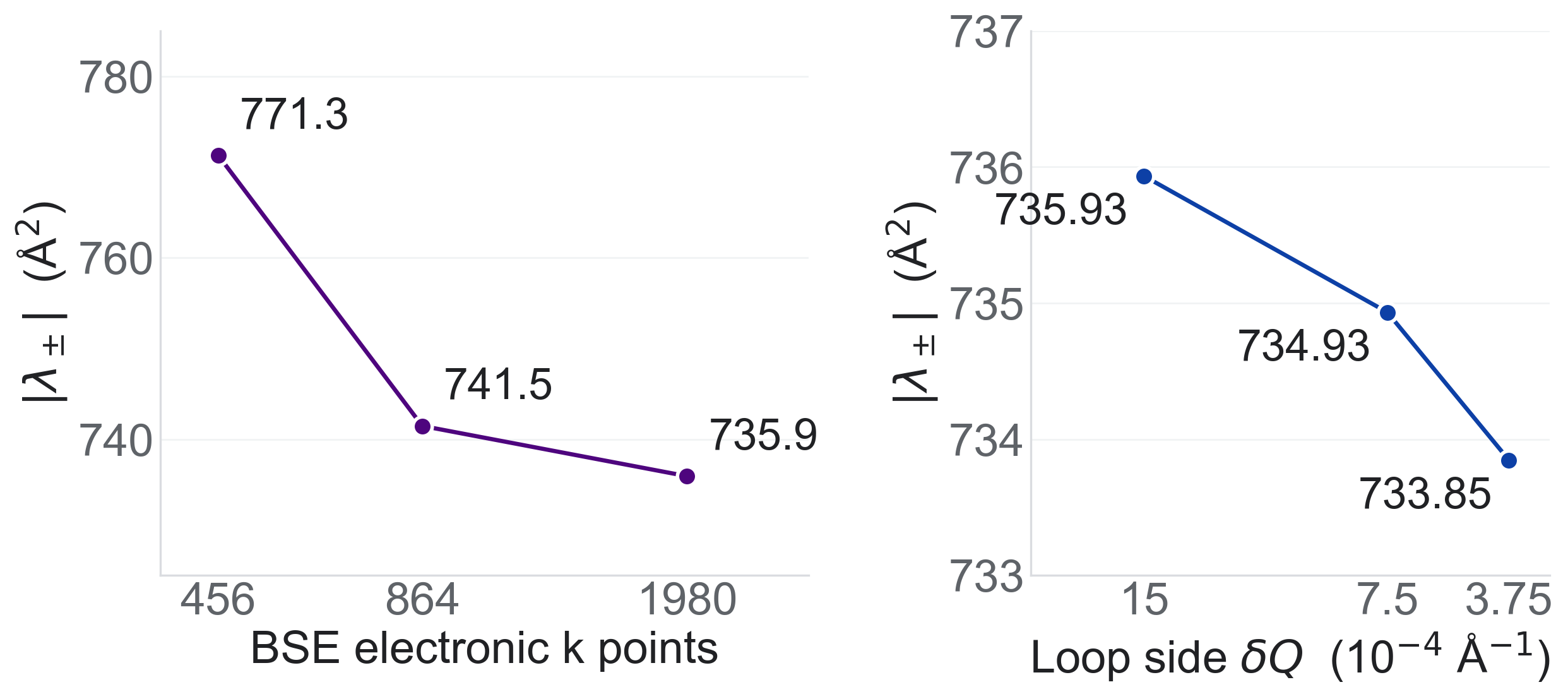
[0:30] Can we trust the number? Refining the grid moves it from about 770 to 740 to 736 square ångström, so the scale is stable, although not converged to the last digit. Random gauge changes leave it unchanged.
[cut if late] What remains are the physical approximations, such as static screening.
For questions: (a) Fixed loop side 1.5 × 10⁻³ Å⁻¹: 771.3 (456 k), 741.5 (864 k), 735.9 Ų (1980 k). The exciton energy over the same refinement goes from 71.0 to 70.0 meV.
(b) At 1980 k, halving the loop side twice: 735.9, 734.9, 733.8 Ų. A finite Wilson loop measures the average Berry-curvature flux through the square; the Berry curvature peaks at Q = 0, so smaller loops approach the local value from above.
Gauge checks: random phases of all Bloch states change the Berry curvature by 6 × 10⁻¹⁰ Ų; random U(2) rotations of the doublet change the eigenvalues by about 10⁻⁹ Ų.
Screening grid level 7 → 8: Δ|λ| ≈ 0.002 Ų, energy 0.003 meV. Exchange sum 19 → 37 reciprocal vectors: Δ|λ| ≈ 0.0006 Ų. Doublet ≥ 9.0 meV below the third state over the whole map. Iterative solver reproduces dense diagonalization.
Not claimed: full k-grid convergence, or survival of the number once static screening, no GW, Tamm–Dancoff and model orbitals are replaced. Convergence within a model is not agreement with experiment.
Results · 6 · interpretation
What we calculated, and what remains open. What we calculated
1. Opposite Berry-curvature eigenvalues for the lowest exciton doublet, λ± ≈ ±730 Ų near Q = 0. Reversing U swaps the valleys (one coarse-grid check).
2. Strong valley polarization: each eigenvalue belongs to a state that is > 99.9 % K or K′.
3. A nearly degenerate lowest doublet, ≈ 9 meV below the next exciton states.
What remains open
4. Global exciton topology. The calculation covers |Qx |, |Qy | ≤ 0.008 Å⁻¹. No Chern number or other global invariant has been calculated.
5. A measurable transport response, such as valley-selective sideways drift: not yet calculated or measured.
6. Device-level modelling: gates, substrate, disorder and a realistic dielectric environment.
In this model of biased bilayer graphene, the lowest exciton doublet has substantial, valley-contrasting non-Abelian Berry curvature. Whether this leads to a global excitonic topological phase or a measurable transport effect remains an open question.
This work · model calculation
Not in the model: GW corrections · dynamic screening · spin–orbit coupling · triplets · phonons and disorder · full ab initio dielectric response · calibrated device environment
19
[0:45] Back to the question. What I calculated: opposite Berry-curvature eigenvalues of about seven hundred and thirty square ångström, strong valley polarization, and a nearly degenerate lowest doublet that is well separated from other states.
What remains open: I calculated the Berry curvature only near Q equals zero, so I have not calculated a Chern number or any global invariant. There is no transport calculation or measurement yet, and no device model. So: substantial, valley-contrasting exciton Berry curvature; topology in the strong sense remains open.
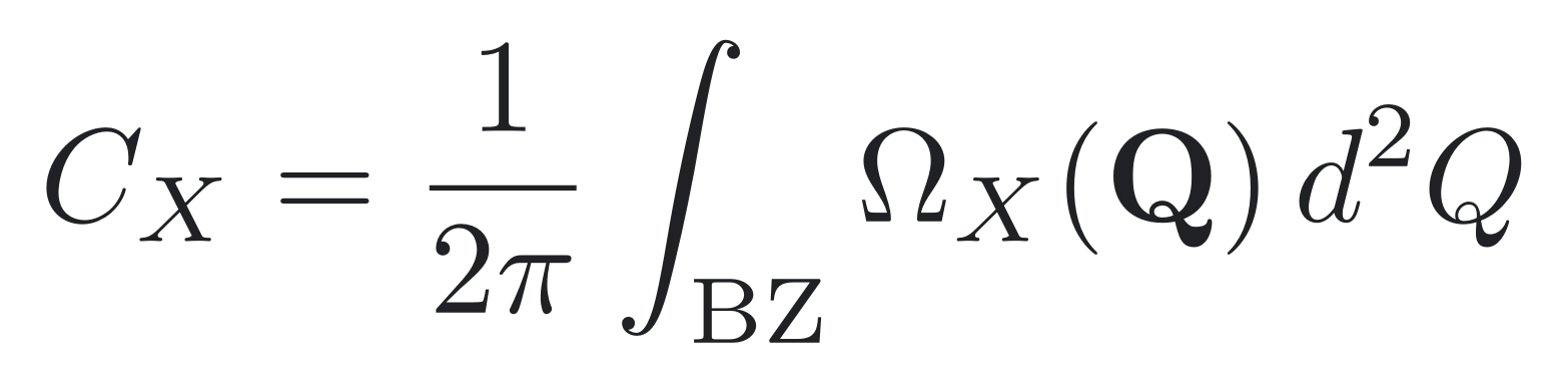
For questions: The trace λ₊ + λ₋ of the Berry-curvature matrix is zero to 6 × 10⁻⁹ Ų on the local map, as time-reversal symmetry suggests. A Chern number of the doublet would be the integral of the trace over the whole exciton Brillouin zone; a local zero does not determine it, and it has not been calculated.
A valley-resolved exciton invariant would need the Berry curvature over the whole exciton Brillouin zone, with the doublet isolated everywhere, or a Wilson-loop spectrum on closed paths.
Bias reversal: tested once, on the 456-point grid. No edge-state or transport calculation, and no measurement.
Not in the model: GW corrections, dynamic screening, spin–orbit coupling, triplets, phonons and disorder, a full ab initio dielectric response, a calibrated device environment. I do not claim a topological exciton insulator.
Towards applications · research directions, not results
Can exciton geometry steer information? A
Valley-dependent exciton transport
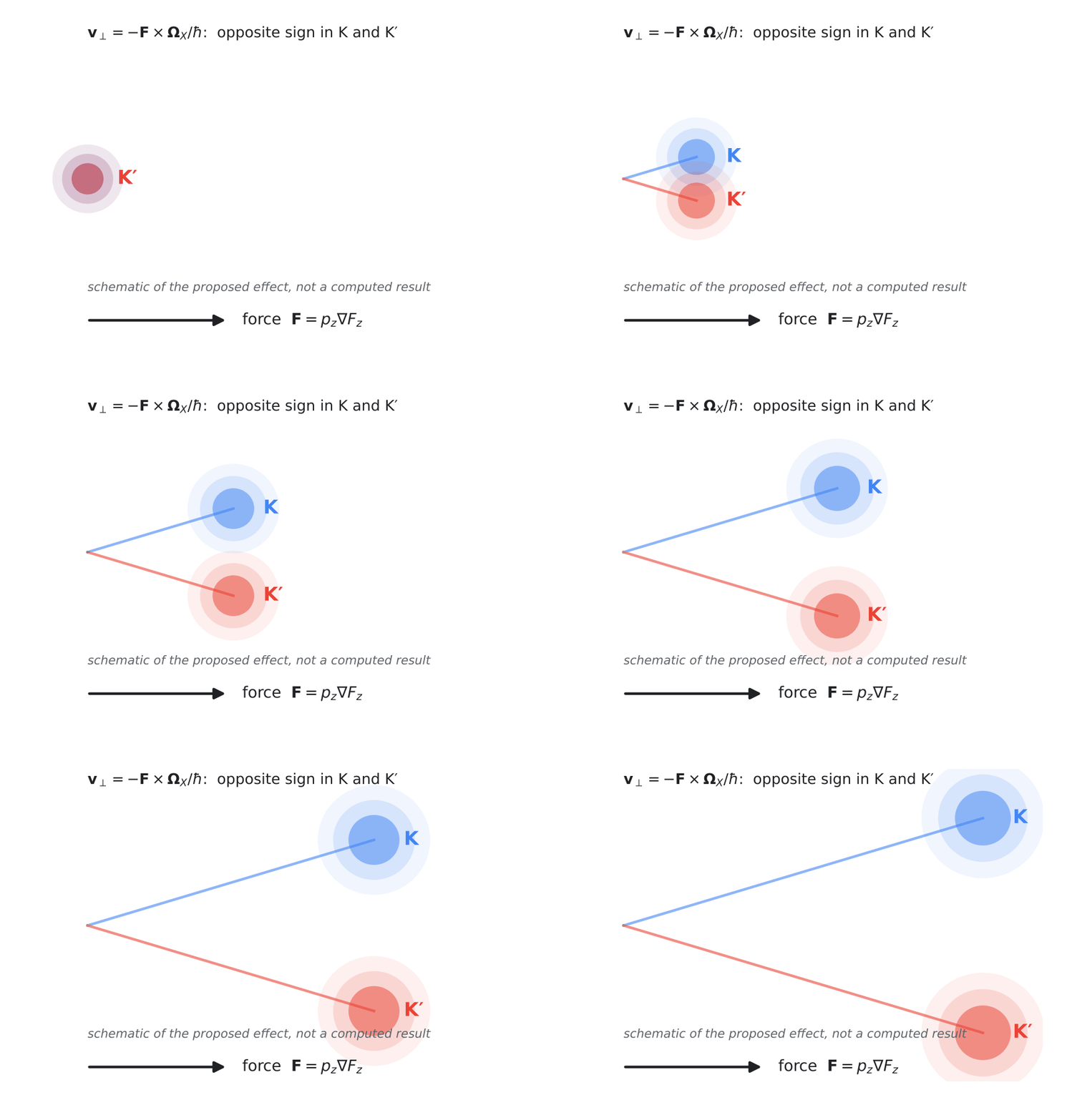
force F (e.g. a field gradient) K′ exciton K exciton prepared Cartoon of the semiclassical expectation. Not calculated.
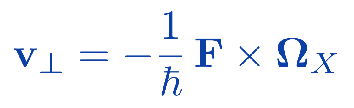
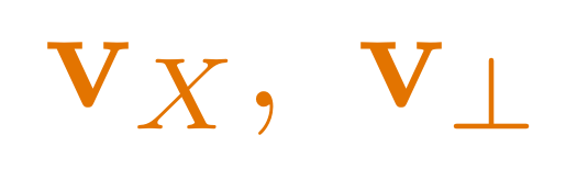
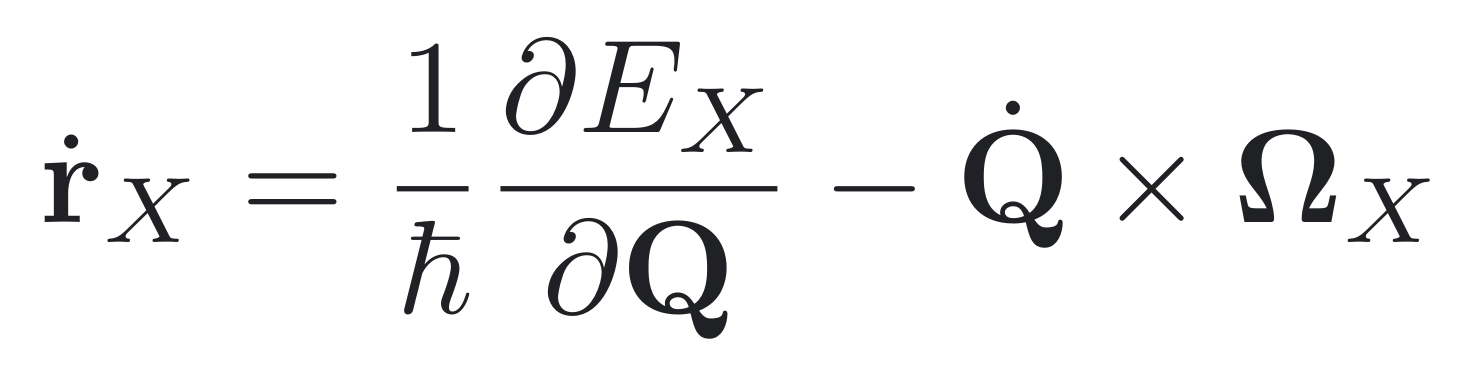
Under a suitable force, Berry curvature adds a velocity perpendicular to the force: opposite in K and K′. For our doublet this needs non-Abelian dynamics.
Would need:
non-Abelian wavepacket dynamics a realistic force on a neutral exciton intervalley mixing and relaxation B
Electrically tunable BLG exciton-polaritons
in-plane momentum E upper and lower polariton , photon , exciton (moves with bias) . Schematic only.
Coupled to cavity photons, these excitons could form polaritons tuned by the gate. Our lowest doublet is optically weak; brighter states may dominate.
Would need:
optical dipole matrix elements light–matter coupling g cavity detuning Hopfield mixing linewidths and losses Proposal · next steps
20
[1:15] Could this ever be useful? These are proposed research directions, not results.
(Left.) Direction A, valley-dependent exciton transport. Under a suitable force, Berry curvature adds a velocity perpendicular to the force. Since the K-like and K-prime-like excitons have opposite Berry curvature, they would drift to opposite sides. Because the lowest excitons form a nearly degenerate doublet, a complete treatment needs non-Abelian wavepacket dynamics, plus a realistic force on a neutral exciton and the rate of intervalley mixing.
(Right.) Direction B, electrically tunable exciton-polaritons. If these excitons couple to cavity photons, the gate could tune the polariton energies. The next calculations would be the optical dipole matrix elements, the light–matter coupling, and the losses.
(Bottom.) Spin and valley transport already work in other materials, and bilayer graphene already works in cavities. Intrinsic exciton Berry curvature in bilayer graphene is the missing piece.
For questions: A: in the semiclassical picture the anomalous velocity is perpendicular to the force and proportional to the Berry curvature. Possible forces on a neutral exciton: a field gradient, strain, or a dielectric pattern. Exchange mixes K and K′, so a valley-polarized packet will not stay polarized; the intervalley coherence and relaxation times decide whether a drift survives.
B: the route of Duarte and colleagues, but starting from these exciton states: optical transition dipoles, light–matter coupling to a given cavity, detuning, Hopfield mixing and linewidths. The lowest doublet is optically weak (slide 12), so brighter states may dominate the coupling. One could then ask whether the polaritons inherit any valley-contrasting geometry, for example in their polarization response.
Context: spin carried 60–92 µm in perovskite and WS₂ polaritons; valley routing in an engineered perovskite lattice; bilayer graphene ultrastrongly coupled to a cavity; Thompson et al. (Nat. Commun. 2025) predict that exciton quantum geometry can enhance diffusion.
Beyond the lab
Ateno AX Robots need a map
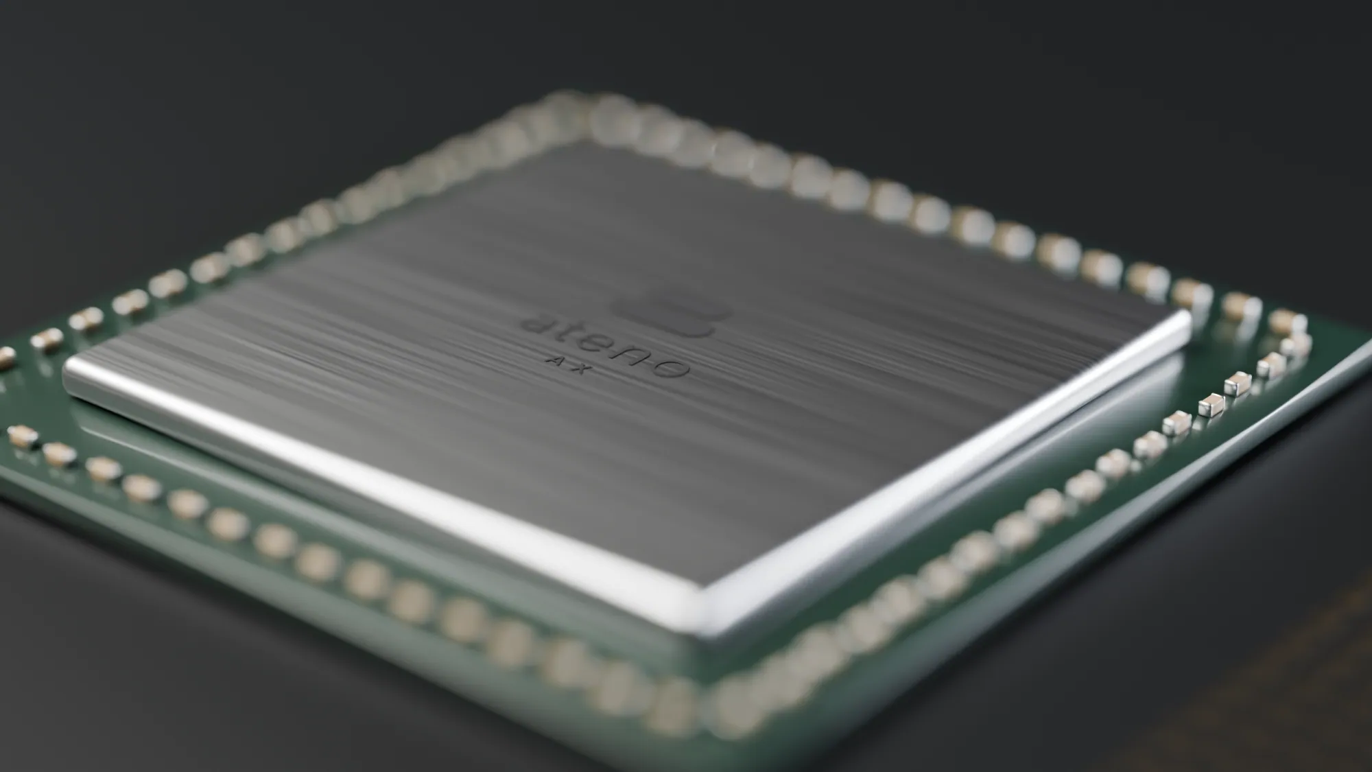
A dedicated chip for on-device 3D mapping: robots and drones build and render Gaussian-splat maps as they move, with no datacenter GPU.
173,161
Gaussians in one 1080p frame on our FPGA prototype
3.9×
faster per frame in 10 days: 1.02 s → 262 ms
Next
silicon tape-out with design partners; no chip yet
Tunnels
Warehouses
ateno.co · Sviatoslav Gladyshev, co-founder & CEO
21
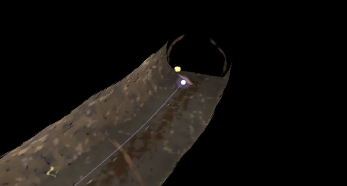
[0:20] Twenty seconds on Ateno, which I co-founded. We are building a chip for on-device 3D mapping, so robots can map places where GPS fails, such as tunnels and warehouses. Our FPGA prototype became 3.9 times faster in ten days; silicon is next.
For questions: Gaussian-splat mapping; the FPGA prototype renders a 1080p frame of 173,161 Gaussians; per-frame time went from 1.02 s to 262 ms. Early stage: no silicon yet; tape-out with design partners is next.
Conclusion
Can we have topological excitons in biased bilayer graphene?
● Established physics: electronic valley Chern numbers that reverse with the bias; bright and dark BLG excitons; room-temperature polariton spin transport; BLG in a THz cavity
● Our calculated results: opposite exciton Berry curvature, λ± ≈ ±730 Ų near Q = 0, for a nearly degenerate, valley-polarized lowest doublet
● Remaining questions: a global exciton invariant, a measurable transport response, and device-level modelling
Thank you.
With thanks to my supervisor, Dr. Marwa Mannai, and CQTS, NYU Abu Dhabi
[1:05] To conclude, back to the question on the cover. Established physics: the electrons of biased bilayer graphene have valley Chern numbers that reverse with the bias, and bright and dark excitons, polariton spin transport and bilayer graphene in cavities are all published. My calculated result: the lowest, nearly degenerate exciton doublet has opposite Berry curvature in the two valleys, about seven hundred and thirty square ångström near Q equals zero. Remaining questions: a global invariant, a measurable transport response, and device-level modelling.
So, can we have topological excitons in biased bilayer graphene? We have found the hidden geometry. Whether it becomes topology is the next chapter of the tale.
Thank you to Dr. Mannai and to CQTS. I am happy to take questions.
For questions: Calculated in a four-orbital, two-valley, finite-Q Bethe–Salpeter model with RPA screening and exchange; stable under gauge changes and grid refinement within the model.
Derivations, convergence tables and checks are in the appendix (slides 24–57).
Foundations and methods
M. O. Sauer & T. G. Pedersen , Phys. Rev. B 105, 115416 (2022).
C.-H. Park & S. G. Louie , Nano Lett. 10, 426 (2010).
E. McCann & M. Koshino , Rep. Prog. Phys. 76, 056503 (2013).
E. McCann & V. I. Fal’ko , Phys. Rev. Lett. 96, 086805 (2006).
R. Yu, X.-L. Qi, A. Bernevig, Z. Fang & X. Dai , Phys. Rev. B 84, 075119 (2011). Wilson loops.
T. Fukui, Y. Hatsugai & H. Suzuki , J. Phys. Soc. Jpn. 74, 1674 (2005).
Exciton Berryology , arXiv:2507.22983 (2025).
Experiments
Q. Shang et al. , Nat. Mater. (2026), doi:10.1038/s41563-026-02782-5.
J. Zúñiga-Pérez & G. Malpuech , Nat. Mater. research briefing (2026).
F. Helmrich et al. , Nature 654, 361 (2026).
Y. Shi et al. , Nat. Mater. 24, 56 (2025).
F. Jin et al. , Nat. Commun. 15, 10563 (2024).
P. Tassan et al. , Light Sci. Appl. 15, 65 (2026).
Z. Jiang et al. , ACS Nano 19, 32123 (2025).
Theory and context
V. G. M. Duarte et al. , Phys. Rev. B 111, 075411 (2025).
J. J. P. Thompson et al. , Nat. Commun. 16, 11448 (2025).
H. Davenport, F. Schindler & J. Knolle , Phys. Rev. B 113, 115102 (2026).
T. Eini et al. , Phys. Rev. Lett. 134, 196903 (2025).
PolArt project , EIC Pathfinder, grant 101130304.
Figures from other work: Sauer & Pedersen (PRB 105, 115416), Helmrich et al. (CC BY 4.0), Duarte et al. (CC BY 4.0), Shang et al. via the Nat. Mater. research briefing (© 2026 the authors).
23
Every entry links to its source. Electronic figures come from my own continuum and lattice models with McCann–Koshino parameters; the exciton figures on the published-physics slides are reproduced from Sauer and Pedersen with attribution. All exciton Berry-curvature numbers and plots are from my own lattice Bethe–Salpeter calculation, generated directly from its saved output files.
The device and polariton papers are grouped as experiments or theory. The WS₂ spin-current figure is from the Nature Materials research briefing, copyright the authors; the bilayer-graphene cavity and polariton figures are reused under CC BY 4.0.
B
Exciton mathematics
Sauer–Pedersen BSE framework, selection rules, exchange, light cone, minivalleys
Back to the start · Optional, for questions
24
Stop here in the main talk. These slides are for questions. Click a section title to jump straight to it. Section C holds every number behind the results slides.
Appendix A · electronic starting point
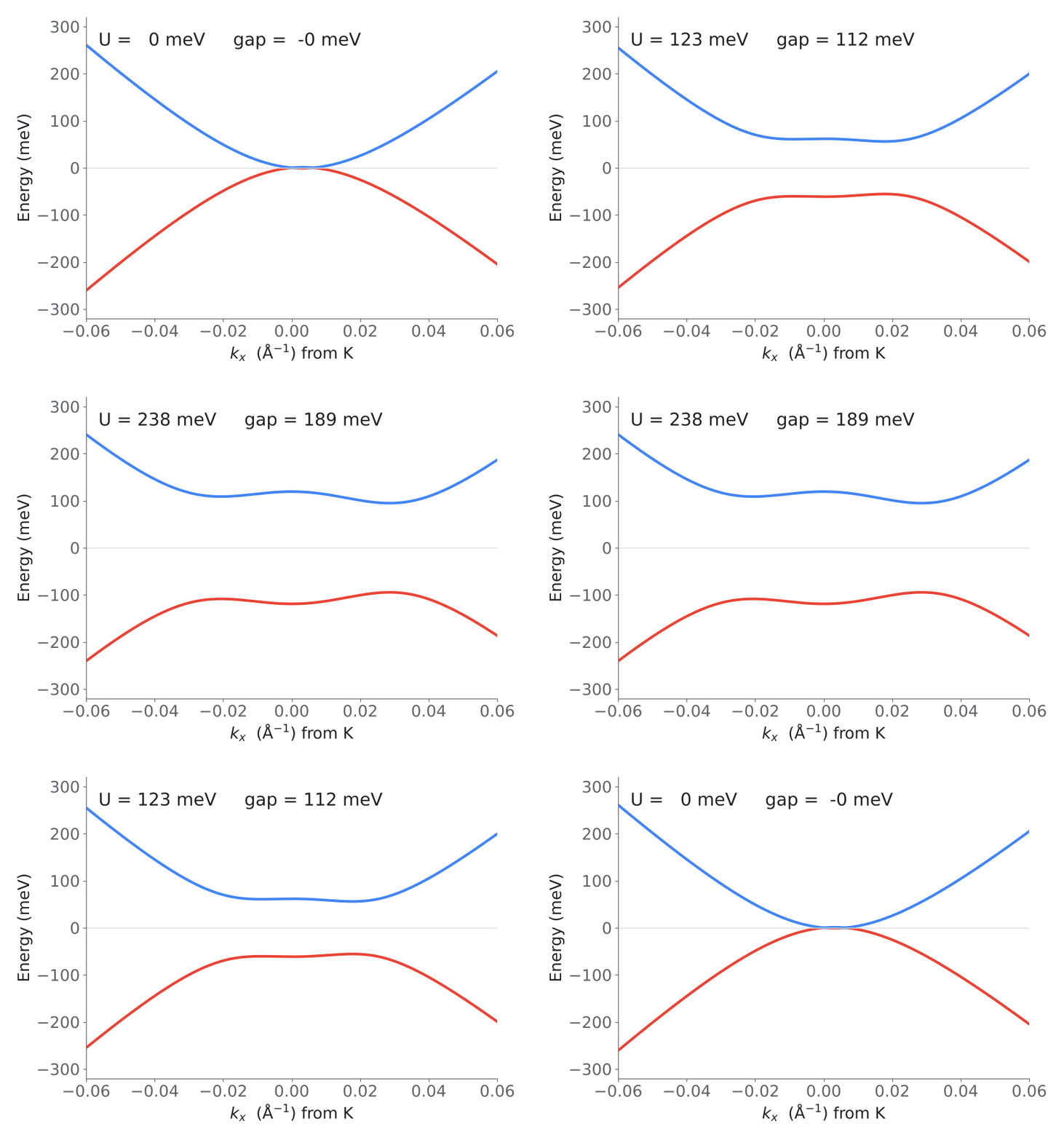
Four bands, then two, with threefold warping.
From four sites to two. The strong interlayer bond removes the dimer sites at low energy.
Threefold warping. Skew hopping turns a circular band edge into a C₃ pattern, which the exciton can feel.
Derived
Appendix A: full derivation · Analytic working calculation, not independently validated
25
We start from the standard four-band model of bilayer graphene and reduce it to two low-energy bands. Skew hopping warps the band edge into a threefold pattern, which matters because excitons are built from these states. This is my own analytic working calculation, and the seven-step derivation is in the appendix.
Derivation · step 0
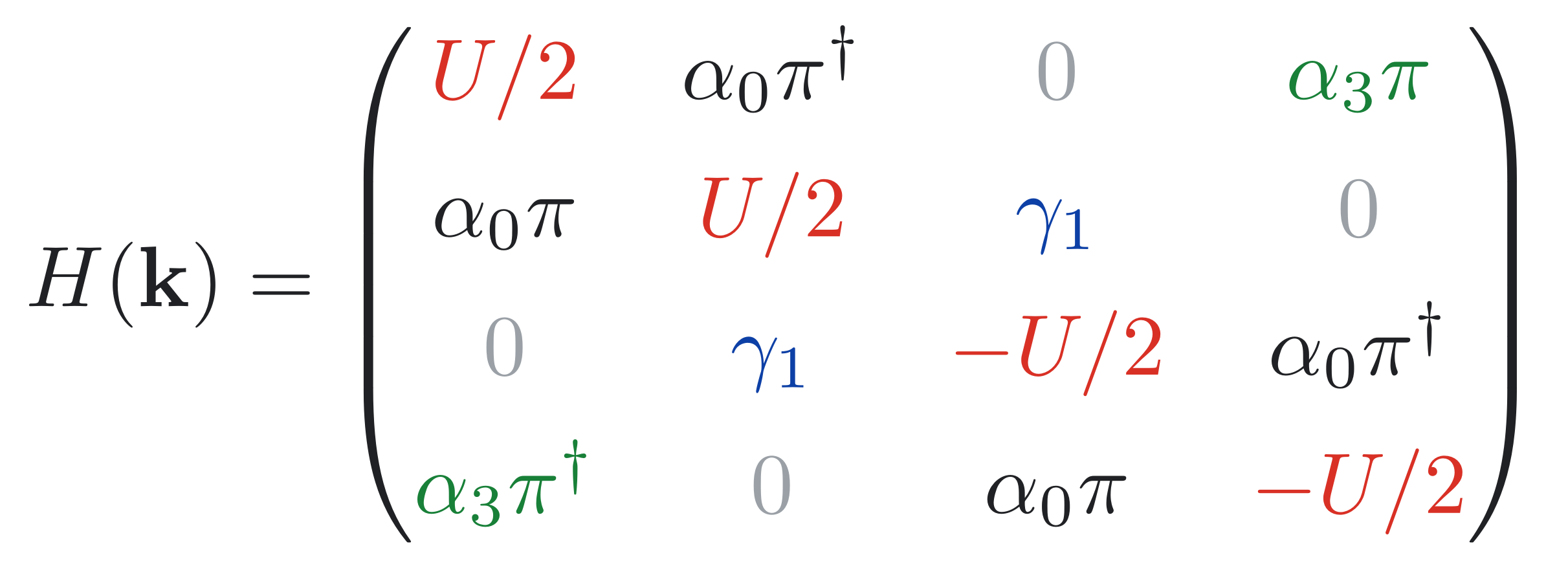
The four-band Hamiltonian.
α₀ intralayer A ↔ B
γ₁ dimer B₁ ↔ A₂
α₃ skew A₁ ↔ B₂
±U/2 layer bias
26
Basis A1, B1, A2, B2 near valley K. Intralayer Dirac hopping alpha0 pi on the off-diagonal blocks, the dimer coupling gamma1 between B1 and A2, the skew hopping alpha3 between the non-dimer sites, and plus or minus U over 2 on the diagonal. K-prime follows by time reversal. Every result in the next slides is derived from this matrix.
Derivation · step 1
Eliminating the dimer sites. Derivation · step 1 of 7
Project onto ℓ = (A₁, B₂); d = (B₁, A₂).
Valid for |E|, |u| ≪ γ₁ ≈ 0.4 eV.
Only path: A₁ → B₁ ⇒ A₂ → B₂.
27
The dimer sites B1 and A2 are pushed to plus or minus gamma1 by the strong interlayer bond. Eliminating them with a Schur complement and expanding to leading order in E over gamma1 gives an effective two-band Hamiltonian on the non-dimer sites A1 and B2. The only second-order path is A1 to B1, across the dimer bond, then A2 to B2, which produces the quadratic term minus alpha0 squared over gamma1 times pi-dagger squared; the skew hop gives the linear alpha3 pi term directly.
Derivation · step 2
Spectrum and threefold symmetry. Derivation · step 2 of 7
Polar form, π = k e^{iθ}.
Two windings interfere: e^{iθ} and e^{−2iθ}.
Gap Δ = 2√(u² + |h|²) ≥ |U|.
The same cos 3θ survives the exact 4 × 4 problem.
γ₃ = 0 removes θ entirely: C∞.
28
Writing pi = k e^(i theta), h has two terms with different winding. Their interference gives the cos 3 theta term in |h| squared, which is the analytic origin of trigonal warping. The exact four-band secular equation is quadratic in E squared, and its constant term contains the same cos 3 theta piece, minus 2 gamma1 alpha3 alpha0 squared k cubed cos 3 theta. Because cos 3(theta + 2 pi/3) = cos 3 theta, the spectrum is invariant under 2 pi/3 rotations only: C infinity is reduced to C3. With gamma3 = 0 the angle drops out of the determinant altogether.
Derivation · step 3
Where the bands touch. Derivation · step 3 of 7
29
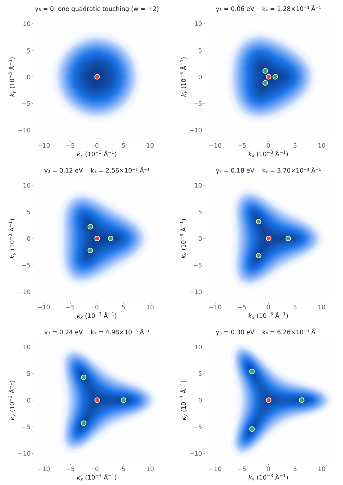
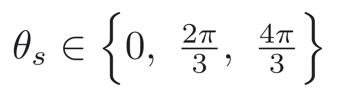
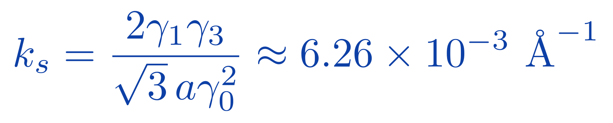
At zero bias, a band touching requires h = 0. Factoring out k e^(-2i theta) leaves alpha3 e^(3i theta) = beta k. Since k is real and positive, e^(3i theta) = 1, so theta = 0, 2 pi/3, 4 pi/3, at radius k_s = alpha3/beta = 2 gamma1 gamma3 over root 3 a gamma0 squared, about 6.26 times 10^-3 inverse angstrom. Together with k = 0 this gives one central and three satellite Dirac points, plotted on the right.
Derivation · step 4
Winding numbers, computed. Derivation · step 4 of 7
Pseudospin d = (Re h, −Im h).
Linear term dominates as k → 0.
w = sgn det J for a linear node.
γ₃ redistributes, never changes.
30
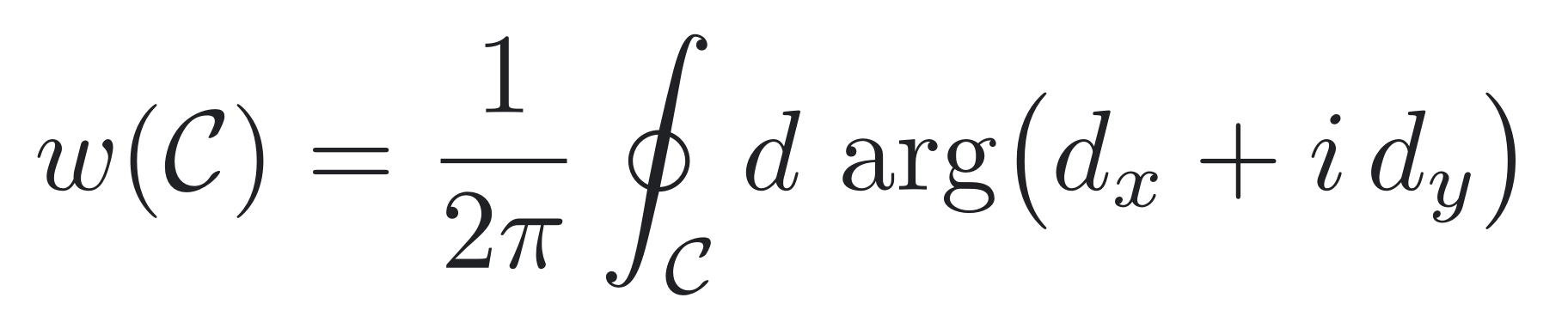
Definition: the winding number counts how many times the pseudospin vector d rotates as k goes once around a contour. Without gamma3, d = minus beta k squared (cos 2 theta, sin 2 theta); the numerator of the winding integrand is 2 beta squared k^4 and the denominator beta squared k^4, so w = +2 exactly. With gamma3, near k = 0 the linear term dominates, d is approximately alpha3 (kx, -ky), which rotates clockwise: w = -1. Expanding around the satellite at (k_s, 0), the constant terms cancel because beta k_s = alpha3, and the Jacobian is diag(-alpha3, -3 alpha3) with positive determinant, so w = +1. C3 maps the satellites onto each other preserving orientation. Total: -1 + 3 = +2.
Visual · winding
Watch the pseudospin wind.
Computed from h(k) of the effective two-band model
31
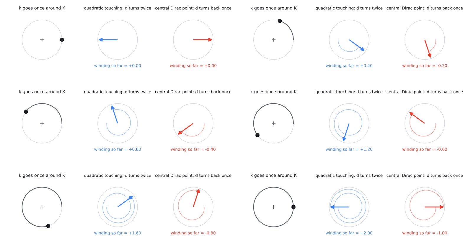
Animation of the winding numbers derived on the previous slide. Left: k goes once around K. Middle: for the quadratic touching (gamma3 = 0), d = -beta k^2 (cos 2 theta, sin 2 theta) turns twice in the same direction: w = +2. Right: near the central Dirac point with gamma3, d is approximately alpha3 (kx, -ky), which turns once the other way: w = -1. The counters show the accumulated winding.
Derivation · step 5
Berry curvature in closed form. Derivation · step 5 of 7
Standard result for H = d · σ.
From ∂d over k: J(k) = 4β²k² − α₃².
Triple product = u (4β²k² − α₃²).
Numerator odd in u, denominator even.
Sign-changing ring: the lobes.
32
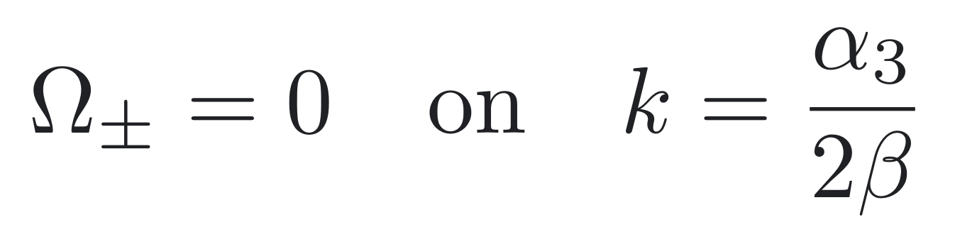
For a two-band Hamiltonian d dot sigma, the Berry curvature is minus-plus one half d dot the cross product of its momentum derivatives over |d| cubed. With d = (alpha3 kx - beta(kx^2 - ky^2), -alpha3 ky - 2 beta kx ky, u) the cross product has only a z component, 4 beta^2 k^2 - alpha3^2, and the triple product is u times that. Hence the closed form. Two corollaries: the Berry curvature is odd in U, so reversing the bias reverses the valley Hall response while the energies are even; and the Berry curvature changes sign on the ring k = alpha3 / 2 beta, which is where the lobes in the Berry-curvature animation come from.
Derivation · step 6
Valley Chern number, integrated. Derivation · step 6 of 7
γ₃ = 0: the Berry curvature is θ-independent.
Elementary antiderivative.
Time reversal: net Chern number = 0.
33
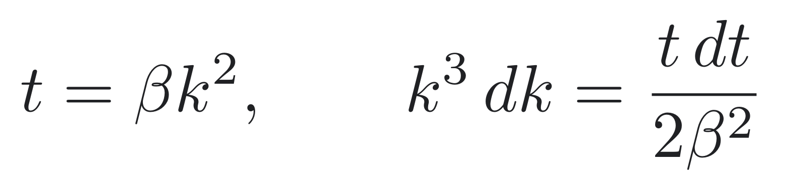
Integrate the Berry curvature over the plane at gamma3 = 0, where it is independent of theta. The angular integral gives 2 pi; the radial integral is minus-plus 2 u beta squared times integral of k cubed over (u^2 + beta^2 k^4)^(3/2). Substituting t = beta k^2 turns it into minus-plus u times integral of t over (u^2 + t^2)^(3/2), whose antiderivative is minus 1 over root(u^2 + t^2). Evaluated from 0 to infinity this gives minus-plus u over |u|, so C = minus-plus sgn U. K-prime has the opposite sign by time reversal, so the net charge Chern number vanishes; what survives is a valley Chern number.
Derivation · step 7
Why γ₃ cannot change it. Derivation · step 7 of 7
The gap never closes as γ₃ is switched on.
Fixed by the winding at large k.
Each massive Dirac node contributes ∓ w/2.
Central + three satellites.
34
Two independent arguments that trigonal warping leaves the valley Chern number unchanged. First, topological: for nonzero bias the gap 2 root(u^2 + |h|^2) is at least |U| everywhere, so turning on gamma3 is an adiabatic deformation, and the Chern number is fixed by the asymptotic winding, w infinity = 2, giving minus-plus sgn u. Second, local: each massive Dirac point contributes minus-plus w_D over 2 times sgn u. The central point (w = -1) gives plus-minus one half, the three satellites (w = +1) give minus-plus three halves; the sum is minus-plus sgn U, the same answer. These are two-band results; the four-band values remain predictions to be checked with a converged four-band integration.
Excitons · equations
The exciton, as an equation. Exciton maths · step 1 of 4
A superposition of e–h transitions.
Kᵈ: screened attraction. Kˣ: exchange.
Interlayer: 2d ≈ 3.48 Å apart.
Brightness is a coherent sum.
Bound below the continuum.
35
Note on conventions: this slide follows the Sauer–Pedersen notation with the electron at k + Q and the hole at k. My own calculation uses the symmetric choice, electron at k + Q/2 and valence state at k − Q/2 (Appendix C). The two labelings are related by a shift of k; the geometry calculation must use one convention consistently, and mine is the symmetric one. The exciton at centre-of-mass momentum Q is a superposition of electron-hole transitions with Bethe-Salpeter coefficients A. The BSE is an eigenvalue problem: band energy differences plus a kernel with a screened direct attraction and a repulsive exchange part. In a bilayer the direct kernel splits into intralayer and interlayer pieces; the interlayer one is softened by the vertical separation 2d of about 3.48 angstroms. The optical matrix element P is a coherent sum of single-transition matrix elements weighted by A, so contributions can cancel (dark) or add (bright). The exciton energy is the gap minus the binding energy.
Derivation · selection rule
Why the ground exciton is dark. Exciton maths · step 2 of 4
Warping allows weak coupling: mostly dark.
Dipole pattern, φ = ∠(q, P).
36
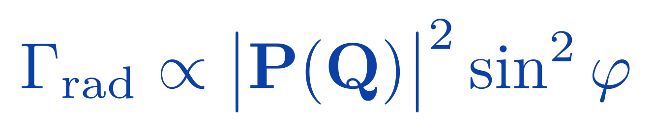
In the rotationally symmetric continuum picture, the exciton carries total angular momentum m = m_pseudo + m_env, with m_pseudo = -2 in K and +2 in K-prime. Normal-incidence light needs m = plus or minus 1. A 1s envelope has m_env = 0, so m = plus or minus 2: forbidden, dark. A 2p envelope with m_env = plus or minus 1 gives m = plus or minus 1: bright. Trigonal warping reduces C infinity to C3, where angular momentum is only defined modulo 3, and -2 is congruent to +1 mod 3, so the coupling is allowed by symmetry but small, set by the warping strength. That is why the ground state is mostly, not completely, dark. The emission rate goes as |P| squared times sin squared phi, the classical dipole pattern.
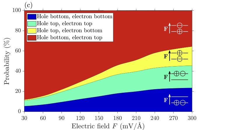
Known · layer structure
Interlayer, anti-aligned excitons.
Mostly hole bottom, electron top.
The dipole points against F. More field means more intralayer weight, larger overlap and a brighter exciton.
Figure: Sauer & Pedersen, Phys. Rev. B 105, 115416 (2022)
37
At low field the anti-aligned interlayer configuration dominates: hole bottom, electron top, dipole opposite to the field, because of the bias-induced charge redistribution. As the field grows, intralayer weight increases, the electron-hole overlap and so |P| grow: this links to the dark-to-bright switch. The field controls the layer composition, hence the dipole, of the composite.
Derivation · exciton dispersion
Light-like excitons from exchange. Exciton maths · step 3 of 4
Eq. (1): intervalley exchange.
Two powers of Q over one.
Linear and parabolic branches.
38
Exchange couples the K and K-prime excitons. Its matrix element is proportional to 1/Q times (Q dot p_K star)(Q dot p_K-prime), where p is the interband momentum matrix element at the valley. The numerator is quadratic in Q and the prefactor removes one power, so the coupling is linear in Q, and the splitting 2|<K|v_x|K-prime>| is linear in Q. One combination becomes light-like, E0 + alpha|Q|, with P parallel to Q; the other is particle-like, E0 + hbar^2 Q^2 / 2M, with P perpendicular to Q. For the dark exciton p is approximately zero, so the same formula predicts almost no splitting, which is what the DFT-BSE calculation finds.
Derivation · emission
Light cone, lifetime, temperature. Exciton maths · step 4 of 4
Only small-Q excitons radiate.
39
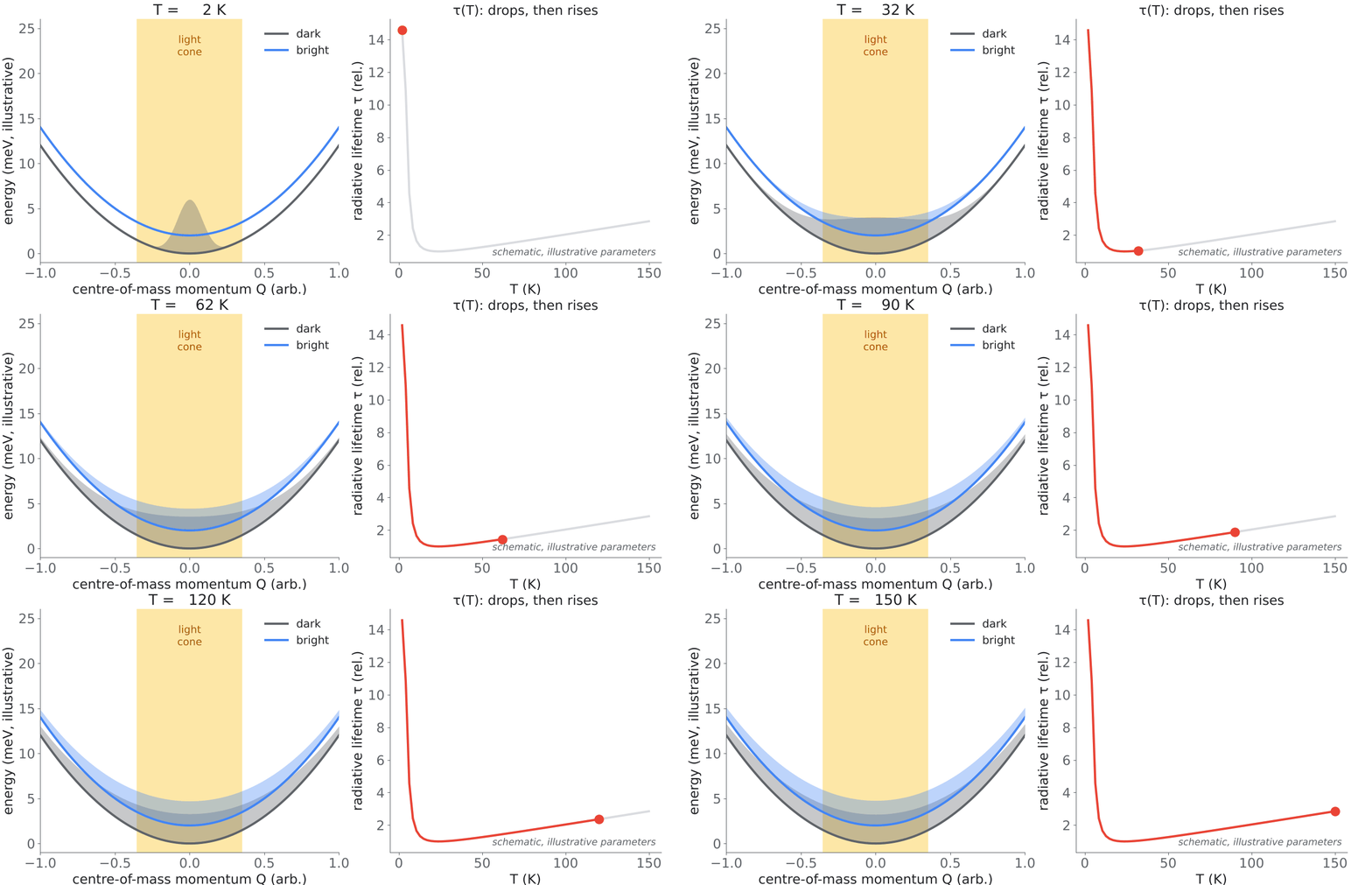
Radiative decay must conserve energy and in-plane momentum, so only excitons with Q below omega over c can emit directly: the light cone. With hbar omega = 0.2 eV and hbar c = 1973 eV angstrom this is about 10^-4 inverse angstrom, a hundred times smaller than the inter-minivalley scale, so the trigonal anisotropy barely matters for emission. The observable rate is a Boltzmann average over exciton bands and momenta; the lifetime is its inverse. With a dark ground state, tau first drops as bright states are populated above the onset temperature (E3 - E1)/4 k_B, then rises again as excitons spread outside the light cone. The emission angle follows from sin theta = cQ/omega.
Visual · emission
Why τ(T) drops, then rises.
Schematic model, illustrative parameters
40
Schematic with illustrative parameters, not the paper data. Left: dark and bright exciton bands with their thermal populations; the yellow strip is the light cone, exaggerated for visibility. Right: the resulting radiative lifetime. At low T almost everything sits in the dark state, so tau is long. As T rises the bright band is populated and tau drops. At higher T excitons spread to large Q, outside the light cone, and tau rises again. This reproduces qualitatively the non-monotonic tau(T) found by Sauer and Pedersen.
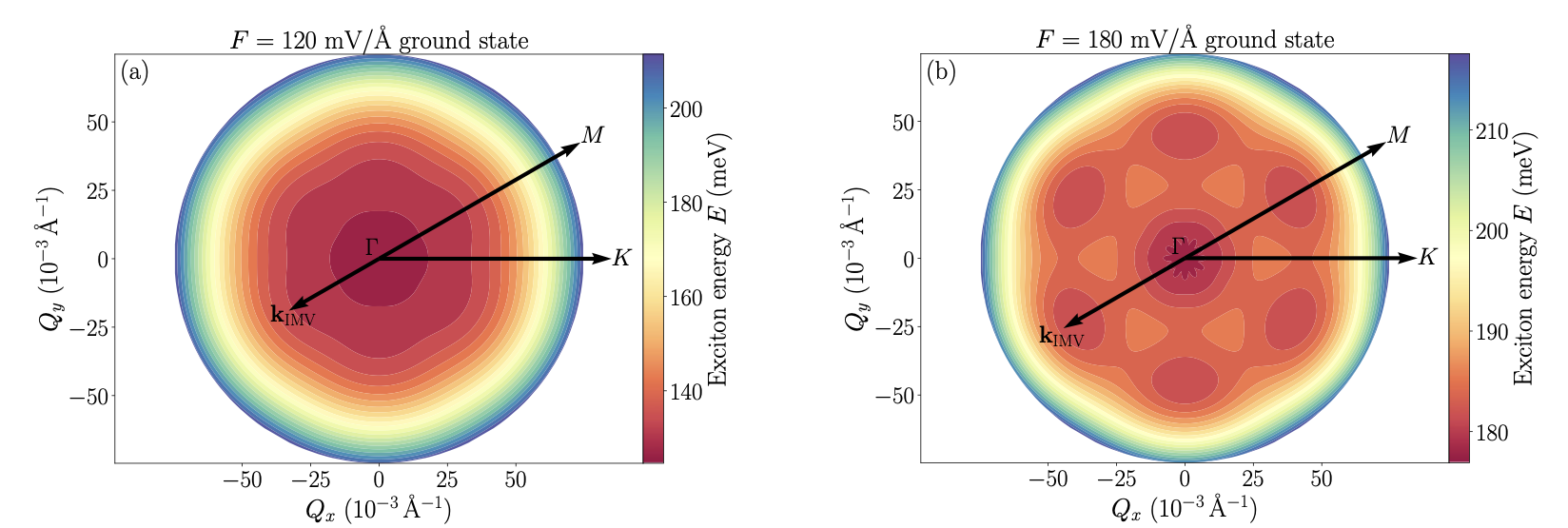
Appendix B · published exciton band over Q
Minivalleys imprint on the exciton band.
Isotropic at 120 mV/Å, trigonal at 180 mV/Å, on the inter-minivalley scale. This is the energy, not yet the Berry curvature.
Figure: Sauer & Pedersen, Phys. Rev. B 105, 115416 (2022)
41
Published
This is the exciton energy plotted against its own momentum Q. The threefold pattern of the electrons shows up in the exciton band at higher field. But this is only energy, so it says nothing yet about exciton Berry curvature, which is the quantity we want.
Appendix C · screening and kernels
Interaction model used in the calculation. Static layer-resolved RPA polarization (2 = spin; both valleys in the k sum)
Screened interaction; e² = 14.3996 eV Å, Gaussian orbital form factor
Direct kernel with orbital embedding (exchange: transition densities, unscreened V at Q + G, 19 G)
Π averaged over six q directions, 110 log-spaced |q| from 10⁻⁵ to 18 Å⁻¹ · no full G, G′ dielectric matrix · no frequency dependence · q = 0 direct term replaced by its cell average (12 × 12 quadrature) · Tamm–Dancoff, singlet only
This work · method
Source: LATTICE_METHOD_RU.md · lattice_bse.py
42
Backup: the interaction model. The polarization Π is computed from the same four-band electronic states as the BSE, at T = 0 for the neutral insulator, resolved into the two layers, with a factor 2 for spin; both valleys are already in the full-zone k sum. V is the bare layer-resolved Coulomb interaction in a uniform dielectric κ = 4.5, with the Gaussian orbital form factor exp(−r_o²q²/2), r_o = 0.6 Å, which sets the short-distance behaviour; it is a model form factor, not an ab initio pz orbital. W = (1 − VΠ)⁻¹V.
Approximations: Π is averaged over six directions of q and interpolated on 110 logarithmic points, so it keeps the dependence on |q| and the layer matrix but not the full angular dependence; the full dielectric matrix in G, G′ is not computed; W is static. No adjustable screening wavevector from my earlier models is used.
Direct kernel: D sums W over reciprocal vectors with the orbital phase factors exp(iG·(τa − τb)), with orbital positions τ = (0, δ1, δ1, 2δ1). Exchange uses transition densities u*_c u_v, the unscreened V and momentum Q + G with 19 vectors G (37 checked); at Q = G = 0 the divergent term cancels by orthogonality of c and v while a finite interlayer term survives.
Appendix C · convergence records
Every run behind the results. Grid refinement (loop side 1.5 × 10⁻³ Å⁻¹)
BSE k RPA level E₁(0), meV threshold, meV |λ|, Ų min link 456 6 71.002 93.20 771.27 0.9976 864 6 70.855 93.51 741.46 0.9985 864 7 70.847 93.51 741.47 0.9985 1980 7 70.019 92.79 735.93 0.9986 1980 8 70.016 92.79 735.94 0.9986
RPA levels 6, 7, 8 = 864, 1980, 5712 electronic k points. The largest BSE is 7920 × 7920.
Loop size (1980 k, RPA 7)
δQ, Å⁻¹ |λ|, Ų valley pol. 0.0015 735.93 — 0.00075 734.93 ±0.99970 0.000375 733.85 ±0.99991
All three loops on the same 1980-point, RPA-7 calculation (the RPA-8 run gives 735.94 at 0.0015).
Coarse 192-point grid: does not resolve the valleys (E₁ = 128 meV, |λ| = 35 Ų, min link 0.44). Used only to test the solver, never as a physical result.
This work · model calculation
Sources: lattice_d5/d6/d7/map/screen8/fine_checks/itercheck_results.json
43
Backup: the full convergence record. All rows are from the JSON output files. The trend with BSE grid is monotonic: 771 → 741 → 736 Ų, with the energy settling near 70.0 meV; the screening grid matters far less than the BSE grid (the two 1980 rows differ by 0.002 Ų and 0.003 meV). The loop-size series shows the finite-loop average approaching the local value. The min-link column is the smallest singular value of the doublet overlap on the loop: always above 0.997, so the subspace is well transported. The 192-point grid is a cautionary example: a coarse uniform grid misses the narrow valleys and gives an unphysical answer (128 meV, 35 Ų), which is why the production grids are dense near K and K′. I did not extrapolate to infinite k-point density, and I do not claim full convergence.
Appendix C · validation
Checks of gauge invariance and numerics. Electronic phase change: exciton energies
3.6 × 10⁻¹⁶ eV
Electronic phase change: Berry curvature
6.2 × 10⁻¹⁰ Ų
Random U(2) rotation of the doublet
≈ 10⁻⁹ Ų
Bloch sewing across the zone boundary
6.1 × 10⁻¹⁵ eV
Recovery of the continuum H near K
1.1 × 10⁻¹¹ eV
Eigenstate residual on the local map
≤ 2.0 × 10⁻¹⁰ eV
Wilson loops rebuilt from stored overlaps
6 × 10⁻¹⁰ Ų
Trace of F on the local map
≤ 5.8 × 10⁻⁹ Ų
Min singular value, doublet, local map
0.99956
Min gap to the third state, local map
9.03 meV
Phase and U(2) checks show the result does not depend on arbitrary choices of basis. They do not test the choice of pair coordinate: the symmetric centre (re + rh )/2 and the orbital embedding τ are fixed conventions, and other conventions define different exciton geometries (Exciton Berryology ).
This work · model calculation
Sources: lattice_validation.json · lattice_local_map_checks.json · rebuild in tools/make_result_figures.py
44
Backup: the individual checks, all from the output files. Re-solving the BSE after random phases on every electronic eigenvector changes the energies only at machine precision, and the Berry curvature by 6 × 10⁻¹⁰ Ų; random U(2) rotations of the exciton pair change the Berry-curvature eigenvalues by ~10⁻⁹ Ų. The Hamiltonian satisfies H(k+G) = D†(G) H(k) D(G) with the orbital phase matrix to 6 × 10⁻¹⁵ eV, and reduces to my continuum Hamiltonian near K to 10⁻¹¹ eV. I independently rebuilt every Wilson loop of the map from the stored raw 2×2 overlap matrices: agreement to 6 × 10⁻¹⁰ Ų.
One important caveat: invariance under phases and U(2) rotations does not mean independence of every convention. Exciton Berry curvature depends on which point of the pair is used as the coordinate — electron, hole or centre — and on the orbital embedding. I use the symmetric centre and the embedding τ = (0, δ1, δ1, 2δ1) throughout; results with other conventions would differ by well-understood terms (see Exciton Berryology).
Appendix C · bias reversal and exchange
Reversing U swaps the valleys, not the pair of values. Run (456 k, loop 1.5 × 10⁻³ Å⁻¹) λ₋, Ų valley of λ₋ λ₊, Ų valley of λ₊ U = +100 meV −771.27 +0.99899 (K) +771.27 −0.99899 (K′) U = −100 meV −771.27 −0.99899 (K′) +771.27 +0.99899 (K) U = +100 meV, no exchange −764.83 +0.999998 (K) +764.83 −0.999998 (K′)
Bias reversal. The unordered pair {−λ, +λ} is unchanged; the valley carrying each sign is exchanged.
Exchange off. |λ| changes by < 1 %: the valley-resolved geometry does not come from exchange; exchange mixes the energy states.
One positive- and one negative-bias calculation on the 456-point check grid. No field dependence λ(U) was computed.
This work · model calculation
Source: lattice_validation.json (standard, reversed_bias, without_exchange)
45
Optional results slide: bias reversal. On the 456-point check grid at loop side 1.5 × 10⁻³ Å⁻¹, U = +100 meV gives λ₋ = −771.27 Ų with a K-polarized eigenvector and λ₊ = +771.27 Ų K′-polarized. At U = −100 meV the values are identical but the valley assignment is swapped: now the negative eigenvalue is K′-like. So the bias reverses the valley-associated sign — just as it reverses the electron valley Chern numbers — while the unordered pair {−λ, +λ} stays the same. This is one reverse-bias test, not a field sweep; I do not draw any curve of λ versus U.
Second check on the same grid: switching exchange off changes |λ| from 771.3 to 764.8 Ų, under 1%, and makes the valley polarization even purer (0.999998). So the Berry curvature belongs to the valley-resolved excitons formed by the direct attraction; exchange's main role is to mix K and K′ in the energy eigenstates, which is exactly why the single-branch Berry curvature comes out near zero.
Appendix C · single states vs the doublet
The subspace is smooth where its states are not. Sorted lowest state: min |⟨X₁|X₁′⟩| on loop
Doublet: min singular value of M
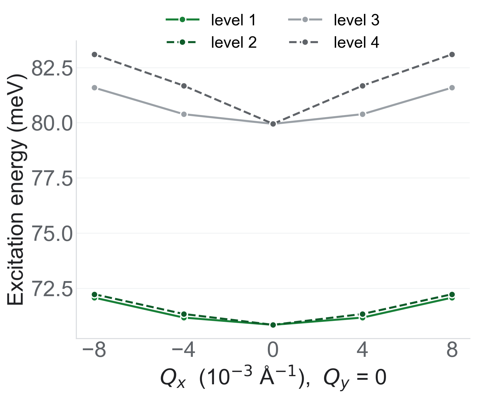
Lowest four levels along Qx (864 k)
Off-centre single branches: |Ω| ≤ 3.5 × 10⁻⁷ Ų. At Q = 0 the single-state link is 0.012, so no single-branch value is reported. Branch splitting: 0.05–0.17 meV.
This work · model calculation
Source: lattice_local_map.npz (864 k, loop side 7.5 × 10⁻⁴ Å⁻¹) · lattice_map_map.npz (dispersion)
46
Backup for results slide 4. Left map: for each small loop, the smallest overlap between the energy-sorted lowest state at neighbouring corners. It is 0.98–0.998 away from the centre, but 0.012 for the loop around Q = 0: there the sorted state jumps, so its Abelian Berry phase is undefined. Right map: the smallest singular value of the 2×2 overlap matrix of the doublet, which is at least 0.99956 everywhere: the two-dimensional subspace is transported smoothly.
Right panel: the lowest four exciton levels along Qx on the 864-point grid. Levels 1 and 2 are split by exchange by only 0.05–0.17 meV on the local map, while the third level is about 9 meV higher. The doublet therefore must be treated as a unit near Γ.
Away from the centre, where single-branch links are healthy, the Abelian Berry curvature of each branch is below 3.5 × 10⁻⁷ Ų — compatible with zero on this grid — in sharp contrast to the ±300–480 Ų eigenvalues of the doublet at the same points.
Appendix C · next steps and open questions
What would turn local geometry into a topological claim. Global
Extend Q over the exciton Brillouin zone; Wilson-loop spectra on closed paths; a valley-resolved invariant where the doublet stays isolated.
Bias
Several U values and a calibrated link between U and the applied field; follow the dark–bright ordering.
Physics
GW energies, dynamic screening, beyond Tamm–Dancoff, triplets, spin–orbit coupling, full dielectric matrix.
Numerics
Finer BSE grids, RPA angular sampling, orbital-radius sensitivity, κ and gate environment.
Observable
Valley-selective anomalous drift needs valley imbalance; estimate its size; ribbon spectra for edge states.
Open
For discussion with Dr. Mannai
47
These are the next steps, in rough priority order, and the questions I would like to discuss.
Global topology first: the present Berry curvature is local. To speak of a topological exciton phase we need the Berry curvature, or Wilson-loop spectra, over the whole exciton Brillouin zone, and we need to know where the doublet stays isolated from higher states; a valley-resolved Chern number only makes sense if the valley decomposition stays well defined.
Bias: repeat at several U values, and connect U to an applied field with a realistic screening model; that also lets us connect to the published dark–bright crossing.
Physics and numerics: the listed approximations, each of which could change magnitudes.
Observable: in a time-reversal-symmetric system the two valleys cancel in any Hall-like response, so an anomalous drift needs valley imbalance, for example from circularly polarized excitation; we should estimate its size. Edge states require a ribbon or domain-wall calculation.
The key distinction
Two different Berry curvatures, one composite.
(a) Electron Berry curvature
One band, over electron momentum k
→
(b) Exciton as a composite
Coulomb binding pair momentum Q
Electron + hole, many pairs mixed
→
(c) Exciton Berry curvature
λ± (Q) of the doublet
Now computed: non-Abelian, lowest two states
Exciton geometry is not inherited from an electron valley Chern number; it was calculated (results 3–4).
(a) derived · (b) schematic · (c) this work
Panel (a): author’s two-band model, U = +100 meV, valley K
48
Concept slide from the proposal, updated. Panel a is the Berry curvature of one electron band over electron momentum k. Panel b is the exciton as a bound composite. Panel c is now computed: the eigenvalues of the 2×2 non-Abelian Berry curvature of the lowest exciton doublet over the pair momentum Q (results slide 3). The key point survives: exciton geometry is a separate quantity and had to be calculated, not read off from electron valley Chern numbers.
Earlier proposal · single-band definition
Exciton Berry curvature, defined. Earlier proposal · superseded
Envelope part plus electron Bloch part; electron at k + Q, hole at k.
Lives in Q-space, not k-space.
Fukui–Hatsugai–Suzuki plaquettes on a Q grid.
Valley-odd, like the electrons.
49
Superseded. This was the proposal before the calculation: an Abelian, single-band exciton Berry curvature with the electron at k + Q and the hole at k, to be evaluated with Fukui–Hatsugai–Suzuki plaquettes. The calculation showed that the lowest exciton states form a nearly degenerate doublet, so a single-band Abelian Berry curvature is not well defined near Q = 0. The actual calculation uses the symmetric pair coordinate and non-Abelian Wilson loops for the doublet (results slides 1 and 4, Appendix C). Kept for the record.
Three transport levels
Three levels, three kinds of evidence.
L1
Diffusion
Density spreads down a gradient. Evidence: spatial spreading in time. No geometry needed.
L2
Anomalous transverse drift
A force bends the path via Berry curvature. Evidence: valley-selective sideways motion that reverses with the force.
L3
Edge transport
A boundary channel tied to an exciton invariant. Evidence: a computed invariant and edge modes that survive disorder.
Which is both calculable in AB bilayer graphene and distinguishable in experiment?
50
Not shown for this project
These three claims are often blurred, and each needs different evidence. Ordinary diffusion needs no geometry at all. Sideways drift needs exciton Berry curvature, and edge transport needs a true topological invariant plus modes that survive disorder. None of them has been shown for this project.
Proposal · observable
What exciton Berry curvature would do. Proposal · step 2 of 2
51
Proposal, not computed · the computed Berry curvature is valley-locked and cancels between valleys unless they are populated unequally
An exciton is neutral, but if it has an out-of-plane dipole then a spatial gradient of the perpendicular field pushes it in-plane. If an isolated exciton branch has nonzero Berry curvature, that push could produce a sideways velocity, like a Hall effect without charge. This is our proposal, the two valleys would cancel unless populated unequally, and the animation is a schematic rather than a result.
Literature
Closest scientific precedents.
Same material. Theory of cavity polariton optics, not exciton topology.
Different platform: moiré multilayer. Precedent for exciton geometry.
Theory: quantum geometry enhances diffusion. Not protected edge transport.
Theory of graphene exciton-polariton collective response.
52
These four papers are the closest work to ours, and none of them is the calculation we propose. One covers the same material but studies polaritons, and another finds exciton Berry curvature on a different graphene platform. The other two are theories of enhanced diffusion and of collective polariton response, which helps define what would be new here.
What could topology add?
Three questions, kept separate.
Berry curvature
Does exciton Berry curvature give a transverse velocity under a force?
Quantum geometry
Can geometric terms enhance ordinary diffusion or drift?
Edge states
Does an exciton band support robust boundary modes?
“Topological” in the strong sense only once one of these is actually shown.
53
Conceptual guardrail: Berry curvature, enhanced diffusion, anomalous Hall-like motion and protected edge states are not interchangeable claims.
The proposal
From electron bands to exciton motion.
Electron bands
→
e–h pairs
→
Exciton band
→
Transport
Earlier proposal. Steps 1–3 are now computed locally (results); the transport step is not. An exciton is not automatically assigned the Chern number of one constituent band.
54
Central research-direction slide, proposed and unverified. Start from the electronic eigenstates, solve the electron-hole problem in the biased four-band basis at finite Q, evaluate the exciton Berry curvature, and ask whether a force produces an anomalous velocity. The pseudospin winding characterises the electrons; it does not by itself determine the exciton Chern number, and an electron valley Chern number does not set it.
Earlier roadmap · before the calculation
From working calculations to a transport claim.
Derived
Electronic baseline
H, warping, winding, Ω(k), Chern: working calculations, Appendix A
Next
Exciton problem
Basis, screening, BSE at finite Q
Planned
Exciton geometry & transport
Lattice Berry curvature, diffusion tensor, edges
Planned
Experiment
Bias-tunable optical or spatial signatures
Risks: basis and screening · valley cancellation · lifetime and disorder · what “topological” means for a neutral composite
55
Step one is a set of analytic working calculations in Appendix A, not independently validated. Step two formulates the exciton problem at finite Q. Step three computes Omega_X with the plaquette method, the diffusion tensor, the anomalous response and finite-edge spectra, benchmarked against limiting cases. Step four compares with bias-tunable optical or spatial signatures.
Context · earlier device slide 1 of 2
Excitons are already being routed and switched.
Working prototype
Bare excitons
Nanoengineered optoexcitonic switch
University of Michigan
Neutral excitons guided and gated in a nanoengineered device at room temperature.
Why it matters: neutral excitons can be routed and switched on a chip-scale structure.
Not: topological transport, and not bilayer graphene.
Jiang et al., ACS Nano 19, 32123 (2025)
Working prototype
Exciton-polaritons
Integrated polariton transistor
IBM Research Europe – Zurich, ETH Zürich, AMO & RWTH Aachen, Wuppertal
2 × 2 µm² device on silicon photonics: picosecond switching, amplification up to 60×, extinction up to 8:1.
Why it matters: exciton-based nonlinearity can be integrated with silicon photonics.
Not: bare excitons, and not explicitly topological.
Tassan et al., Light Sci. Appl. 15, 65 (2026) · arXiv
56
Backup. Why should anyone care whether excitons have band geometry? Because excitons are already being used to carry and switch signals.
Left: the University of Michigan optoexcitonic switch. These are bare excitons: neutral electron–hole pairs that are guided and gated in a nanoengineered structure at room temperature. It is a working prototype. It is not topological and not bilayer graphene.
Right: the integrated polariton transistor from IBM Research Zurich and collaborators. This is a different particle: an exciton-polariton, an exciton strongly mixed with a cavity photon. The device switches in picoseconds with gain, on a silicon-photonics platform. Again a working prototype, but polaritonic, not topological.
Message: excitons carry energy and information without net charge. That makes them attractive for low-loss optoelectronics, but also hard to steer with a voltage. Band geometry is one candidate handle. None of these devices demonstrates topological exciton transport in biased bilayer graphene.
Context · earlier device slide 2 of 2
Topology and geometry are entering exciton physics. In development
Exciton-polaritons
PolArt neuromorphic accelerator
EIC Pathfinder, 2024–2028, coordinated from the University of Warsaw
Aims to build hardware neural networks from polariton microcavities.
Why it matters: a funded effort is testing polaritons for computing hardware.
Not: a finished or commercial chip. It is a research project.
polart-project.eu · CORDIS 101130304
Experiment
Exciton-polaritons
Topological valley polaritons
Nanyang Technological University, Tsinghua University and collaborators
Valley-polarized kink states in a patterned perovskite lattice at room temperature, gap ≈ 9 meV.
Why it matters: topological protection and exciton-based states can coexist at room temperature.
Not: bare excitons, and not bilayer graphene.
Jin et al., Nat. Commun. 15, 10563 (2024)
Topologically enhanced exciton transport
Thompson et al.
Predicts that the quantum geometry of exciton bands can enhance exciton diffusion.
Why it matters: exciton band geometry is predicted to change how far excitons travel.
Not: an experiment, and not protected edge transport.
Thompson et al., Nat. Commun. 16, 11448 (2025)
57
Backup. Three more examples, now closer to topology and geometry. The pills say what each one is: development project, experiment or theory; and which particle: polaritons or bare excitons.
PolArt is a European research project building neuromorphic hardware from polariton microcavities. It is in development, not a product.
The perovskite experiment of Jin et al. shows topological valley kink states of exciton-polaritons at room temperature, with a gap of about 9 meV. This is an experiment, but with polaritons, in a patterned photonic lattice, not with bare excitons in bilayer graphene.
Thompson et al. is a theory prediction for bare excitons: the quantum geometry of the exciton band can enhance diffusion. It is not an experiment and not protected edge transport.
Together: geometry and topology are becoming useful words for exciton and polariton transport. But none of these is a demonstration of topological exciton transport in biased AB bilayer graphene. That gap is what motivates our calculation: first find out whether the exciton states there have geometry at all.